Wednesday January 5th 2005
Finance : eleventh lecture (part two)
Joint random variables and portfolios of securities
Standard model
Two securities studied jointly
Conditional probabilities
Calculation of conditional probabilities
Dependence
A little game of guessing to understand better conditional probabilities
The game with another distribution of probabilities
Independence
Pictures of joint distributions
Theoretical probabilities and estimations from series of outcomes
Scattergrams
Examples of links
Covariance and correlation (a first
glimpse)
It is fundamental that you understand well the standard model of finance that we reviewed in part one : a security S, its price today P, its random value in one year, with a mean and a spread, and therefore its profitability in one year (denoted either R or just X when there is no confusion), with a mean too, denoted rS, and a spread denoted σS.
We denote them r and σ, when there is no confusion.
The spread σ of the random profitability of S (another name for its standard deviation) is the definition of the risk of the security S.
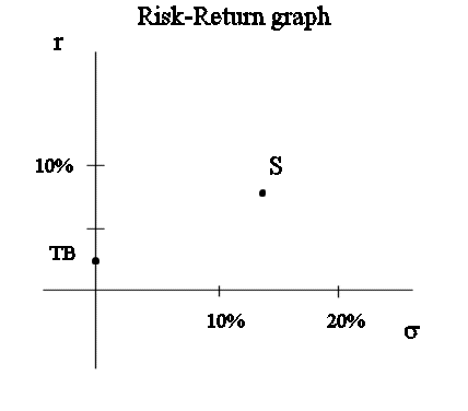
Then each security in the market can be positioned on the risk-return graph.

In the standard model, any stock and bond that you can read about in the newspaper covering a given financial market, for instance the NYSE (the New-York Stock Exchange), has an r and a σ, and can be positioned on this graph for the market.
On the risk-return graph we also positioned the short term Treasury bond, that is the risk free security. It corresponds to the point with abcissa zero and ordinate r0.. The value of r0 as at January 2005, in the US, is 2.25%. The risk free security will play an important role in the theory of portfolios.
Now we shall study the various optimal ways, and non-optimal ways, to invest our money into a portfolio of several securities.
Two securities studied jointly :
To begin with, we look at the profitabilities of two securities produced by the same experiment E ("invest into two securities and wait one year"). Following our habit, let's call these profitabilities X and Y.
Think of them as the profitabilities, for instance, of a Ford stock and an IBM stock.
And to make life simple we consider that each of them can only take three values, the three values studied in part 1.
So the outcome of the pair (X, Y) can be one of nine possible pairs. Suppose from past history of X and Y, or for any other reason, we know the probability of each pair. They are given in the table below :
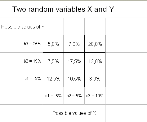
(Don't forget that the outcomes of X and of Y, themselves, are percentages, because X and Y record profitabilities.
A more realistic example would have X and Y each take more than three values, for instance a dozen values for X, a1, a2, ... a12 and a dozen values for Y, b1, b2, ... b12, representing possible profitabilities for X and for Y. Completed with probabilities they would have means and spreads. But this would require to study a table of 144 joint probabilities. And in that case Calculus and continuous densities soon are simpler tools of study.)
We readily see that X and Y are "linked", and positively linked : when the outcome of Y is b1, the outcome of X has more chances to be small too.
To say that X and Y are "linked" (or "dependent") has a very precise meaning. To grasp this meaning we need to introduce the concept of conditional probabilities.
And to grasp the concept of conditional probability let's think once again of a large number of replications of the experiment E, that produced, say, 10 000 pairs of outcomes :
(x1, y1), (x2, y2), (x3, y3), .... .... .... , (x10000, y10000)
We already know the meaning of
Pr{X = a1} = 25%.
It simply means that in the above collection of 10 000 pairs - disregarding entirely what the yj's can be - we have roughly one fourth of the pairs with xi = a1 (and the more numerous replications we have, the closer to one fourth it is).
Now the idea of the conditional distribution of X, given Y = b3, is straightforward :
if we look only at the subset of pairs where Y = b3, within this subset the proportion of pairs such that X = a1 is called
Probability of X = a1 given Y = b 3
and is denoted
Pr { X = a1 | Y = b3 }
Calculation of conditional probabilities :
If we indeed "throw" 10 000 times the experiment E, we will roughly have 3200 pairs where Y = b3.
And, among these 3200 pairs, 500 will also have X = a1.
So Pr { X = a1 | Y = b3 } = 15,6%.
(We often use the idea of "a large number of replications of E", because then the actual frequency counts are also the exact "underlying" probabilities.)
The definition of Pr { X = ai | Y = bj } is

If the distribution of probability of X changes when we condition on a value of the outcome of Y, then we say that X and Y are "linked" or "dependent".
And this is the case here, because we had
Pr{X = a1} = 25%
and we also have
Pr { X = a1 | Y = b3 } = 15,6%
When we know that Y was b3, then the probability that X be small has changed, because within the subset of pairs where Y = b3, the distribution of probabilities of X is not the same as the general one (the general one is also called "the marginal" distribution of X disregarding what Y is).
A little game of guessing to understand better conditional probabilities :
To better grasp the usefulness of the conditional distributions, let's play the following little game :
You and me know the experiment E and the distribution of probabilities of X and Y.
I produce an instance of E, and therefore a pair of outcomes of X and Y.
I don't tell you what the outcomes are, and you are asked to guess what X was. (We disregard entirely what Y did.)
To make the game more attractive, let's say that you win $1 if you guess right, and you don't lose anything if you guess wrong :-). And we shall play the game many times.
How to best guess X ? (In a more an inflated language : "What is you best playing strategy ?")
Answer : look at the marginal distribution of X (25%, 35%, 40%), and therefore always guess X = a3.
It may look stupid, but if we play this game 1000 times, you will finish with around $400 in you pocket.
Any other "strategy" will earn you less.
For instance if you decide to guess randomly with probabilities 1/3, you will end up with only $333 in your pocket.
And if we try to be "sophisticated" and guess randomly with probabilities 25%, 35% and 40%, we will end up with $345.
Let's enrich the game a bit : now before you guess what was X, you are allowed to ask "what was Y ?"
Will you want to ask this question ?
Will you even be ready to pay a little bit for the answer to this question ?
Answer : YES.
Why ?
Because then you can improve you guessing strategy.
For instance each time Y turns out to b1, you will no longer guess X = a3, you will guess X = a1.
Each time Y is b2, you will guess X = a2.
And each time Y is b3, you will guess X = a3.
Then your expected gain, in 1000 games, will be
31% x $403 + 37% x $473 + 32% x $625 = $500
So, in fact, you should be willing to pay up to 10 cents for the extra information in each game.
The game with another distribution of probabilities :
Suppose now the random variables X and Y have the following joint distribution of probabilities :
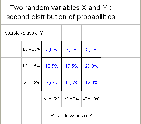
In this case, playing the same game of guessing X, is any information on Y useful ?
Answer : NO
Will you pay for information on Y ?
Certainly not !
Why ?
Because the conditional distributions of probability of X, given Y has such and such value, do not change from its marginal distribution.
Let's check for X = a1 :
Pr { X = a1 } = 25%
Pr { X = a1 | Y = b1 } = 0,075 / (0,075 + 0,105 + 0,120) = 25%
Pr { X = a1 | Y = b2 } = 0,125 / (0,125 + 0,175 + 0,200) = 25%
Pr { X = a1 | Y = b3 } = 0,050 / (0,050 + 0,070 + 0,080) = 25%
Exercise : Check for the other possible values of X.
In the second example above, X and Y are said to be independent.
The conditional distributions of probability of X given Y equal anything do not change from the marginal distribution of X.
We also say that Y carries no information on X.
This happens if and only if the rows of probabilities in the above table are all proportional. (In which case this is also true of the columns of numbers.)
And this happens if and only if for any index i and index j :
Pr { X = ai and Y = bj } = Pr { X = ai } x Pr { Y = bj }
that is the probabilities of joint events involving X and Y, are equal to the product of respective probabilities concerning X alone and Y alone.
Definition : When for all i and j we have
Pr { X = ai and Y = bj } = Pr { X = ai } x Pr { Y = bj }
we say that X and Y are independent.
The natural character of this definition appears once again if we think of a large number of replications of E : if we produce 10 000 pairs of outcomes
(x1, y1), (x2, y2), (x3, y3), ... ... ... (x10000, y10000)
Pr { X = a1 } is the proportion of pairs where x is a1.
If X and Y are independent, if we select only those pairs where y equal, say, b2, it should not change, within that subset, the proportion of pairs where x = a1.
And this happens if and only if, for all i and j, we have
Pr { X = ai and Y = bj } / Pr { Y = bj }
(that is the proportion calculated in the subset where y = bj)
=
Pr { X = ai }
(the marginal distribution of X)
Pictures of joint distributions :
Just like we pictured distributions of single random variables

we can picture joint distributions of RV.
The first example above (where X and Y were "dependent", or "linked") is this :
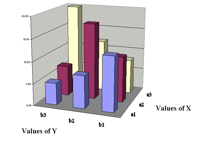
And the second example above where X and Y were independent is this :
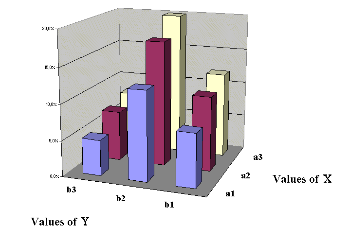
Here we see clearly the proportionality of rows and columns, which is the condition of independence.
Theoretical probabilities and estimations from series of outcomes
As was already explained in lesson 2 there are four types of situations where we deal with randomness :
| We know everything about the probabilities | We only know a past series of outcomes | |
| Discrete random variables |
|
|
| Continuous random variables |
|
|
This is true whether we deal with single RV or with several RV studied jointly (that is, produced by the same experiment, and that usually are not independent).
In this session, until now, we were in the left column, and in the top row : case of discrete joint RV's and where we know the theoretical probabilities "driving" the occurences of outcomes.
As before, the more realistic case in when we don't know the "underlying probabilities" (another name for "theoretical probabilities") but we have a past series of outcomes at our disposal. If the past series of outcomes is large enough, it provides us with reasonable estimates of the underlying probabilities.
In the case of one RV this was the role of a histogram : it estimated the underlying frequency distribution of the RV.
In the case of two RV's studied jointly, the extension of the histogram is the scattergram. It records the past series of outcomes (of pairs) we have at our disposal, and it provides reasonable estimates of the underlying joint probabilities.
Just like we constructed histograms by counting occurences of outcomes of X in various intervals, we can construct a scattergram of X and Y from a collection of pairs of outcomes. Here is a result for another pair of RV - not the same as above :
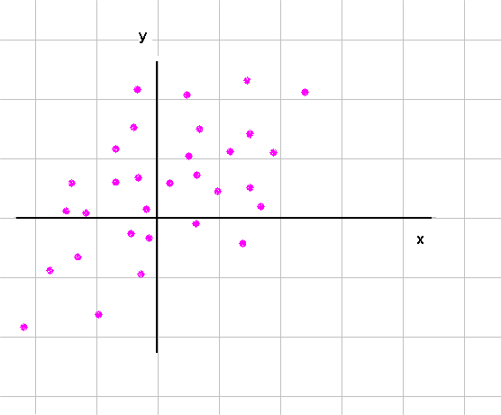
From this we can count pairs in cells of the grid :
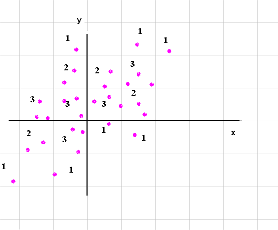
And we can draw a three dimensional estimate of the joint density of X and Y :
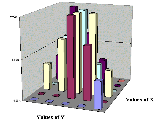
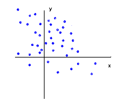
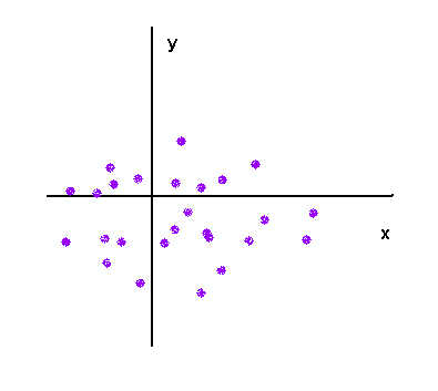
We see clearly, once again, that here X and Y are not independent. They are positively linked, which means that they tend to vary in the same direction : when X is small, Y tends to be small ; and when X is large, Y tends to be large.
In fact this can readily be seen from the first scattergram :

Mild negative link :
No link (independence) :
Strong positive link :
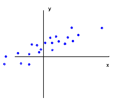
A point to note : the fact that X and Y are strongly positively linked has nothing to do with the slope of the swarm of points, but is related to the fact that it is almost a straight line.
(A second point : if the relationship between X and Y was a regular curve with a simple shape, but not a straight line, then probabilitiy theory would not be appropriate to study the link between X and Y.)
Covariance and correlation (a first glimpse) :
Next time we shall study the mathematical tools to deal with the degree of dependency between two random variables.
One concept, extending the concept of variance of X, will be introduced : it is the covariance of X and Y.
Without surprise you may already guess that it will be :
Covariance (X, Y) = Expectation of { [ (X - E(X) ] times [Y - E(Y) ] }
We will see the nice properties of this measure of the linkage between X and Y.
And next to the covariance of X and Y, we will define the correlation of X and Y : it is just the covariance "rescaled" by the two standard deviations.
Correlation (X, Y) = Covar (X, Y) / σX times σY
Correlation (X, Y) is denoted : ρXY
These are all the tools necessary to identify optimal portfolios of securities and suboptimal portfolios of securities.