Elementary finance

The concept of probabilities

Text

introduction
the two ultimate situations
events without cause
equiprobable events
example of 10 000 rolls of a die
why we observe a rough equality of experimental frequencies
explanation with three flips of a coin
other physical probabilities: fully known wheel of chance
unknown wheel of chance
theoretical probabilities underlying any random experiment

What is disconcerting about probabilities is that we make statements about the future which are not firm, and yet are useful.

Probability theory never makes firm statements about future observations, only about their level of probability. It is indeed a strange way to describe the world.

The situations under consideration always boil down to either of two cases:

1. when there is some symmetry or equivalence among the possible outcomes of an experiment, none in particular should surprise us more than any other
   
   
2. on the other hand, for instance, when we have one red ball in an urn, and a large number of black balls
   
   
   and we pick one ball "at random", we can safely plan on picking a black one.

But this "safely plan" does not exactly have the same sense as something sure.

So, another disturbing aspect of probabilities, to a rational mind, is that we deal with events without cause. Yet, once again, we shall derive many interesting and useful things about them.

We cannot build the usual logical string of events which leads to explaining why we got outcome x or outcome y. Even Einstein exclaimed "God doesn't play dice!" to express his uneasiness with such modelling of the world.

However, not only probability theory is useful in many fields (insurance, finance, construction...) but in atomic physics it appears to be a fundamental ("ontological") feature of the world (or at least of our descriptions of it, if we want to venture into the philosophical discipline called phenomenology...).

Equiprobable events.

When we have an experiment and a random variable X which can have outcomes { a₁, a₂, ... a_m } and the a_i's show symmetry (like with a die), then we define the probability of each a_i as 1/m,

If we roll the die many times, we can observe that each outcome { 1, 2, ... 6 } will roughly appear one sixth of the times.

So this is a vindication of the meaningfulness of "attaching theoretical probabilities" 1/6 to each possible outcome of the die.

You can find nice simulations of rolling a die (and dice) at https://www.stat.sc.edu/~west/javahtml (item "a central limit theorem applet").

Example of 10 000 rolls of a die:

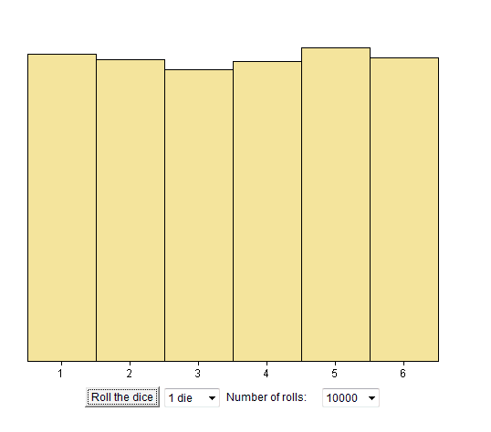
With the simulation offered on the aforementioned site, we rolled a die 10 000 times. And we counted how many times we got 1, how many times we got 2, ... how many times we got 6. Here is the plot of the results

(the vertical axis is a count of the outcomes of each possible value read on top of the die)

We see the rough equality of experimental frequencies of each outcome.

Moreover, this illustration of the rough equality of experimental frequencies, is itself an illustration of the second case we mentionned at the beginning of the lesson:

in this urn

you can "safely" assume that you won't pick the red ball.

Why 10 000 rolls is of the same nature?

Answer: if we consider the experiment = [ 10 000 rolls of one die ], we have 6¹⁰⁰⁰⁰ possible outcomes (an outcome is one series of 10 000 results).

And it so happens that most of them have more or less equal frequencies of 1's, 2's, ... 6's.

We just picked one!

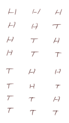
To get a feel of this fact, look at 3 flips of a coin. Here are the 8 possible series of 3 flips:

Observe that "most of them have more or less as many heads as tails".

Of course, we could do some calculations about numbering, binomial law, Chebyshev's inequality (none of it is very difficult), and prove this result. But the teacher believes that too much proof obscures the understanding rather than sheds light on what's going on.

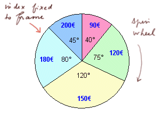
To many other devices, we can attach "physical probabilities" like we did with a die or a coin. Here is a "wheel of chance", with sectors and payoffs, and an index fixed on the frame. Spin the wheel and see what payoff is pointed at.

(download a spreadsheet simultating the wheel of chance)

To the sectors of the wheel of chance, we attach probabilities proportional to the angles. It is a variant of equiprobabilities: think of the disc split into 360 angles of one degree. Each has the same probability 1/360. Then one sector being pointed at by the index is just an event with probability equal to its angle / 360.

Let's consider now the case of an unknown wheel of chance. Suppose I have a wheel of chance, with sectors and payoffs, but you don't know the values (neither the probabilities nor the cash flows).

We can still play the following game: you pay a ticket, we spin the wheel, and you win the payoff shown.

If we play many times, you can figure out the possible outcomes, and estimate their probabilities, although you don't know the "theoretical" probabilities.

In any random experiment, we shall consider that there are some theoretical probabilities underlying the experiment, and attached to each possible event. Sometimes, we can actually know them (from physical considerations of symmetry or such like). But most of the times we don't know them. A past history of results of the experiment, however, will be useful to estimate them.

This will be the case when operating in the stock market. The basic experiment is "buy a security (or several securities) and wait one year". We won't know the "theoretical" probabilities underlying the experiment, but past history of prices will be useful.

Caveat: the history of prices of one security will not be a sequence of outcomes of one RV, but the history of profitabilities (from one year to the next) will.

Screens of the video

Course table of contents

Contact