Elementary finance

Modelling of time

Text

introduction
in practice time is continuous
example of continuously compounded interests
discrete time model
yearly cash flows
continuity and discreteness in mathematics
continuity and discreteness in physics
summary

As we saw, time plays a fundamental role in finance. So we need to say a few words about the way we shall treat it in our equations to calculate present values.

In everyday life, time is treated as a continuous variable, and so it is also in practice in finance.

• It is possible to lend money for a very short period of time
• For instance, banks lend money overnight (usually to other banks, in order for the borrower to abide by the rules, in force in the monetary zone where they operate, about reserves of cash)

It leads, for example, to calculations of continuously compounded interests. Here is the way it goes:

Suppose I lend you a sum of money M for a period of time d, using simple interests, with the rate r (over the whole period d). This means that we agreed that at the end of d, you will owe me

Everyone is familiar with this equation for the calculation of simple interests.

But, suppose now we agreed to compute the repayment due like this: I actually lent you the sum M over two periods of length d/2. And at the end of d you owe me

because at the end of d/2 you owe me M( 1 + r/2 ), which you keep, so at the end of the second period of length d/2, you owe me the sum calculated above.

We may also agree to split the period d into n subperiods of length d/n, in which case the repayment due becomes

A mathematical result establishes that when n tends to + ∞, the coefficient next to M tends to e^r, which is written with the usual mathematical notations

where e = 2.71828183... It is actually one of the definitions of the number e, which plays such an important role in mathematics (alongside π and a few other constants).

This leads to the formula for "continuously compounded interest" : if r is the simple interest rate for a unitary period d, then if you borrowed a sum M, and we agreed on continuously compounded interests, the repayment after a period t is Me^rt/d. Taking d as the unit of time (measured by 1) this writes

Notice that r is no longer the interest rate (in the sense of the calculation M( 1 + r) ) of any continously compounded loan. It is just a parameter to which we give the name "simple interest rate" over the time period of length 1.

In this course in elementary finance, however, we shall not use continuous time. Time will consist of discrete steps of 1 year.

The modelling with discrete time is for the sake of classroom explanation.

In a first approach, discreteness is simpler to handle than continuity.

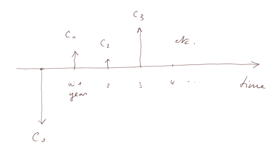
So the cash flows produced by a security or by an investment will be like this

C₀ will be the initial expenditure, a positive number, appearing with a negative sign in calculations of NPV. In the case of the purchase of a security, it will more usually be called P.

Paradoxically, in more advanced mathematics (and more advanced finance), continuity turns out to be easier to manipulate than discreteness.

A digression on physics.

Energy was naturally considered a continuous quantity, until 1900 when it became necessary to model it as a physical variable taking only discrete values in order to explain certain phenomena.

The same may happen to time in future physics.

To summarize:

• we shall consider discrete time
• this is for the sake of simplicity in explaining elementary finance
• in a more advanced course, time will of course be a continuous parameter

Screens of the video

Course table of contents

Contact