Elementary finance
The modelling of uncertain future
Text
introduction
sure and unsure future values
case when the future value X is a known sure figure
price of any sure bond
no arbitrage principle
application
case when X is an unsure figure
future price of a share of stock
three approaches to forecasting stock prices
elementary probability theory
basic random experiment
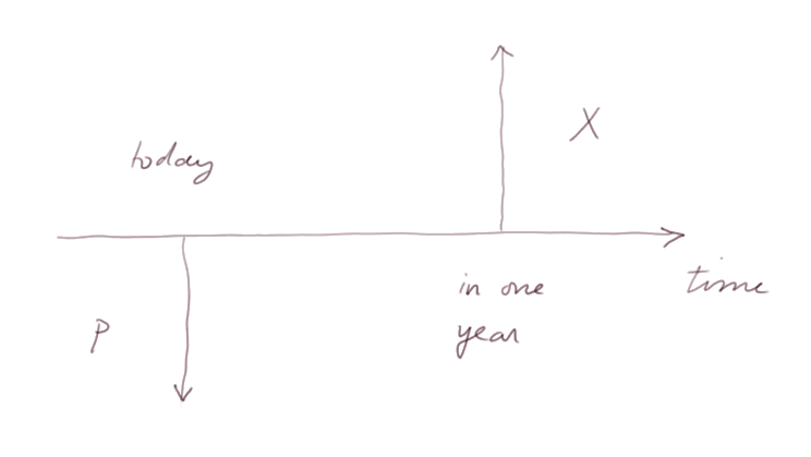
For a while, we shall concentrate on investments with a single future cash flow in one year,

The tools and analyses we shall present apply both to financial investments and to physical investments. So we shall not specify whether we are dealing with one kind or the other.
Time, as we said, will be discrete, and we shall therefore look at one time step.
So we are in one market, with one currency unit, and discrete time with steps of one year.
The model, of course, is simple and rudimentary, but it is sufficient to explain the origin and workings of the fundamental financial concept of discounting.
There are two types of investments as pictured above:
- those where the cash flow X in one year is a known sure figure
- those where the value of X, viewed from today, is an uncertain (or unsure) figure
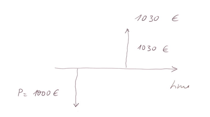
When we buy a bond S issued by a strong creditworthy borrower, the payment we shall receive in one year is a sure figure, known at the time of the purchase of the bond.
For instance, when we buy for, say, PS = 1000 € a 1-year 3% bond from the government of a strong developed country, we know that in one year we shall receive X = 1030 €.

A consequence of the no arbitrage principle (see below) is that any sure bond T producing a known value Y in one year must have today a price PT in proportion of the price PS of the above bond, the proportion being Y / X.
where r0, in the example, is 3%.
Generally speaking, r0 is called in elementary finance the "no risk" or "zero risk" rate.
Let's spell out in detail the no arbitrage principle and its application to the example.
No arbitrage principle: in the same market, two identical products cannot have different prices.
Indeed, suppose it was the case. Think of a market where two grocers at two different stalls sell the same salads with two different prices, 2€ and 1.8€. And in front of both there is a queue of clients.
Then buy salads at 1.8€ and open a third stall next to the stall selling salads at 2€, and sell them also at 2€ (or if you prefer at 1.9€). You have created a money making machine. But the law of supply and demand, which here for once applies perfectly, will necessarily level out the various prices.
Application to the example of bonds:
Think of a sure bond T which will produce in one year a value Y = 854 €.
The bond T is identical to the bond S rescaled with the factor Y / X. So its price must be the price of S rescaled with this factor. Hence
PT = 1000 x ( 854 / 1030) ≈ 829 €
If you are ill at ease with considering fractions of a bond S, then consider 829 bonds S. They are identical to 1000 bonds T, since both are sure, and produce the same value in one year. Therefore they must have the same value today. So T must be worth 829 €.
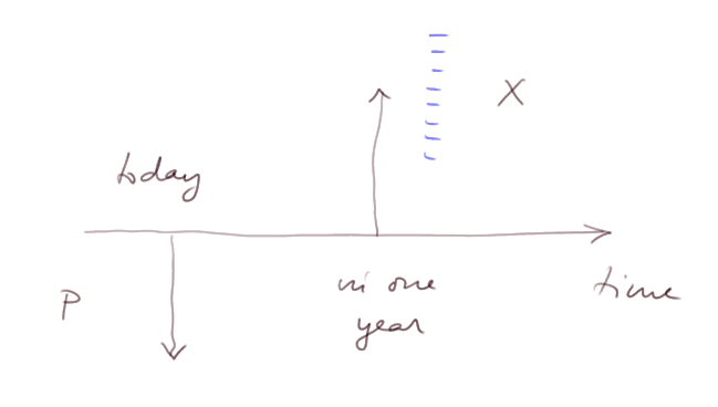
In most investments (financial or physical), the value we shall get in one year is unsure. By this we mean that at the time of the investment, we don't exactly know what will be the future value X we will obtain.
It can be represented like this:

where the blue dashes suggest that X will take a value in a range of values.
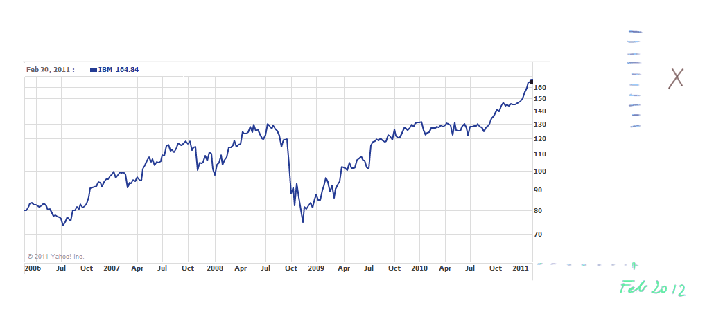
For instance, if I buy today (February 21st, 2011) one IBM stock, I will pay today $164.84.
But I don't know what will be the cash I can get from this share in one year (reselling price, plus possible dividend in the meantime).

There are 3 approaches to get an idea of the price of IBM in one year:
- probability theory
- chartist analysis
- Graham-Dodd-Buffett analysis of the firm
The Graham-Dodd-Buffett approach says: "Don't pay much attention to past prices. Study in depth the firm itself, its products, markets, management, perspectives. And if you find that today's price is too low compared to the cash flows the firm will produce, buy." It does not use probability theory. But it still uses discounting.
The chartist approach claims to be able to foresee the short term evolution of prices from certain shapes displayed by the stock prices in the past. We are not familiar with this approach, and don't grant it much value anyway.
In this course, we shall use elementary probability theory.
Even if it has limited application in the long term (historical events like uprisings, or defaulting by governments, or earthquakes, are hard to forecast with dates), it works reasonably well in the short term.
And it provides a clear and strong justification for discounting.
Buy a stock and wait one year will be the "random experiment", like "throw a die". So we shall devote the next few lessons to a review of elementary probability theory.
Screens of the video
|
|
|
screen number display zone |
Course table of contents
Contact