Wednesday October 20th 2004
Finance : second lecture (part one).
Two important ideas
introduced in lesson 1
A major
difference between Finance and Accounting
Today we shall
study some simple random variables
The randomness of securities
Elements of probability theory
Caveat : in Finance we meet percentages in two quite different instances
The four types
of situations in which we study RV
A
wheel with sectors, specifying payoffs, simulating a security
A different example : a continuous RV, where we don't know the "underlying
probabilities"
Wheel with sectors (cont'd)
Difference between "knowing all the probabilities" and "knowing only a past
history of outcomes"
Possible values, and series of outcomes of a random variable
Expectation of a random variable
Simple averages and weighted
averages
Link between the expectation E(X) and the simple average of the xi's
To summarize
The usual representation of the possible values of X and their probabilities
More on expectation of X
Becoming accustomed
to financial calculations
The different aspects
of mastering a field
Exercise
Two important ideas introduced in lesson 1
Among the important ideas introduced last time are the following
If I have today $100 of money, it is not the same thing as having a piece of paper promising $100 in one year. Indeed the promise-bearing-piece of paper is worth today less than $100. We don't pay $100 for it today. If the promise is absolutely risk-free, in the US today the price of such a bond is $100/(1 + 1.75%) = $98.28 .
If the promise is risky, its price today is even less than $98.28 . To compute its price P we discount the average future payment by a discount rate r higher than 1.75% . To determine, depending on the security, what is the proper r will be one of the central topics of this course.
A major difference between Finance and Accounting :
Distinguishing between the value today of a security and the amount of money it promises to pay in the future is an important difference between Finance and Accounting. In Accounting, on the Assets side of a balance sheet, we record debtor papers at the value they promise to pay. For instance if a client gives us an IOU promising to pay us $50 000 in six months (this may happen ; some clients are very slow payers and yet we like to keep them - like the French state) we record today a value of $50 000 entering our firm. We do not discount it like finance people do. We could ; but it would make Accounting even more intricate, with not much gain in terms of usefulness to view the assets and liabilities of the firm. We know that accounting is already quite approximate (for instance keeping the value of land at its historical cost), but we prefer robustness to deceptive accuracy.
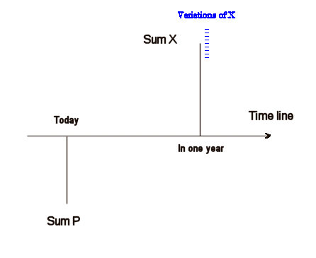
So, the standard situation in Finance is this : we are offered to purchase today a security S promising to pay us in one year a sum of money X, which incorporates some randomness ; what price P should we pay for S today ? The answer will depend upon the probabilistic characteristics of X.
If X has an average value of $110, P = $100 may be a good price, may be not. If X has an average value of $101, we know that P = $100 is too high. On the other hand if X varies between $200 and $300, P = $100 sure is a very good price !
Today we shall study some simple random variables.
We need to study elementary probability theory to understand clearly Finance. Most MBA textbooks in American universities skip this step, claiming that "everybody knows probabilities". The consequence is that they become at times very confusing. In particular, when studying past portfolios random profitability we don't always know what is exactly the experiment that can be reproduced they have in mind. For example talking about the random character of the risk-free rate requires some care...
So today we shall study this :

This is not the standard representation of the variations of a random variable X. We shall see the standard representation in a little while.
The randomness of securities :
We need some theory about random variables because the value and therefore the yield of securities in the future are random variables.
For example I can open the newspaper, look at the financial pages and read the price of a General Electric share, on the NYSE (New York Stock Exchange) market, yesterday, quoted in euros (in my newspaper) : 26.66€. I can read the price the day before : it was 26.89€. I can read the highest price over the past twelve months; and the lowest price over the same period. But the price it will reach in one year, I have no idea. It is not written in the paper !
Well, when I say "I've no idea" it is not quite true. I can guess it won't be 75€ (unless GE announces a fantastic new discovery in the next months...), nor 5€. In fact I have the whole past history of GE stock price as useful information about the random variable. I also have all the information published by GE in its annual reports, in the documents filed with the SEC (Security and Exchange Commission) and elsewhere, about its activities. I have whatever information I can gather about its markets, its competitors, the technologies it employs, its management.. And I have financial analysts' opinions...
What drives the price of a stock ? Answer : essentially it is the prospects of dividends in the future. Indeed, investing boils down to relinquishing money today in order to get more money in the future. Buying a stock means "buying future dividends". One may add "and buying a future resale price", but the resale price is "future dividends" for the new buyer as well. So a stock is only a promise of an unending series of dividends. It is close but not identical to a bond, which is "buying a finite sequence of coupon payments (= yearly interest payments), plus finally the initial value back". This is a bond extending over several years, as opposed to lending money over only one year. But the idea is exactly the same. We shall devote a whole lesson specifically to bonds.
Many financiers, like for instance Warren Buffett, the most famous American investor of the last half century, study carefully all the information they can get about firms listed on the stock market in order to appreciate whether, in their view, their market price is correct, or overvalued, or undervalued, and to make their investment decisions.
Most often, rather than look at the price, we prefer to look at the profitability of a stock from one year to the next. A stock which had a price of $23 in mid 2003, and which sells for $27 in mid 2004, has a profitability, in 2004, of 4/23 = 17.4% .
Elements of probability theory :
The random variables we shall encounter in Finance take real values in a continuous range, what are called "real numbers". For example, the future value of a security may take all possible values between $30 and $200. Or the profitability of a portfolio might take all possible values between -70% and +250%.
Caveat : in Finance we meet percentages in two quite different instances.
Do not mix up the two.
To begin with, it is easy to think of random variables which can take only a finite set of possible values. We saw, for example, dice. They can take only six values. Random variables that can only take a finite range of values are called discrete and finite. There exist a type that is discrete but not finite, but that is of no use for us in this course.
We shall study discrete RV and continuous RV.
We shall also consider two fundamentally different situations : situations where we know everything about the probabilities of the possible values of the RV, and situations where we do not know the exact probabilities, but we have access to some past history.
So there are four types of situations we shall study.
The four types of situations in which we study RV :
| We know everything about the probabilities | We only know a past series of outcomes | |
| Discrete random variables |
|
|
| Continuous random variables |
|
|
The situations in the (pink) column on the left are less often encountered in reality, but are easier to study at first, to understand probabilities. The situations in the (green) column on the right are more frequent, but at first they are a bit less simple to study.
We start our study of probability with an example from the top left cell : a discrete RV, all information about the probabilities of the outcomes of which is known.
The values of the outcomes will be numbers (amounts of money). Therefore we will be able to talk about average values and other computations with the outcomes.
Note that not all RV take numerical values : if I draw a card at random from a deck I can draw a queen, or a 7. There is no concept of average value for a hand made of queen of heart, king of spade, 10 of spade, 8 of diamond and 5 of diamond.
A wheel with sectors, specifying payoffs, simulating a security :
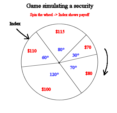
Consider the following device and game

The game is simple enough : spin the wheel once. When it stops the black "Index" points to a sector. We win the payoff inscribed in red in the sector.
This creates a nice simple random variable X (the payoff) that is very easy to understand.
X can take five possible values :
a1 = $70
a2 = $80
a3 = $100
a4 = $110
a5 = $115
It is customary to note the possible outcomes of a discrete RV X : a1, a2, a3, ... ap .
And because we know the size, in degrees, of each sector, we know the probabilities of each possible outcome of X.
Pr{X = a1} = 30°/360° = 8.33%
Pr{X = a2} = 70°/360° = 19.44%
Pr{X = a3} = 120°/360° = 33.33%
Pr{X = a4} = 60°/360° = 16.67%
Pr{X = a5} = 80°/360° = 22.22%
So we are in the situation of the top left cell.
The hand out gives you the yearly profitability of a portfolio made of large US industrial stocks over 73 years, from 1926 (included) until 1998. Technically, it is called the Standard and Poor's composite index. Let's call this random variable : R. Every year R takes a value. We see that the outcomes vary from -43.76% (in 1931) to 53.12% (in 1933).
We can think of each year as "a replication of the experiment producing R".
We don't know exactly the probabilistic behavior of R. This means that we don't know exactly, for instance, the probability that R be greater than or equal to 30%.
But we have a past history of outcomes for the random variable R. And these are valuable.
Now we are back in a situation where we know exactly the probabilistic behavior of the random variable. This is a big difference from above. Here having a past sequence of outcomes of X does not add any useful information.
Now comes a question that will stimulate our intuition : How much should we be willing to pay to play this game ?
Obviously if the ticket price to play the game is $60, it is fine ! And conversely if it is $150, it is not fine.
But what about $80 ? At first glance it looks... probably OK.
$90 ?
$100 ?
$110 ? Well, this seems too expensive now. We are likely to loose money on average...
More in a little while. But first let's stress again the following point.
Difference between "knowing all the probabilities" and "knowing only a past history of outcomes" :
When we know all the probabilities Pr{X=ai}, because we know the sizes of the sectors, we are not particularly interested in knowing, on top of that, a sequence of past outcomes of X. We will definitely not pay to acquire such a piece of information in order to increase our chances to win. Because we already know everything that can be known about X.
On the other hand, think of another wheel, similar but not identical to the one above, with sectors and payoffs. Let's call the new random variable : Y. Suppose I tell you the possible payoffs of Y, but I don't tell you the sizes of the sectors. (I hide this new wheel.) In this case, if I offer to tell you a past sequence of 1000 outcomes of Y you will definitely be interested ! In this case this further information has value.
That is the big difference between situations in the left column and situations in the right column of the four possible situations.
(Well in practice things are not always as simple as in theory and there are people who go to casinos and study for a long long time the results of the roulette game, even though the probabilistic behavior of the roulette, in theory, is perfectly known, and past history is therefore useless. Some of these people, like an old professor of probability of mine, even become banned from entering any casino... :-) Why ? Because first of all there are some games at the casino where it is possible to actually win in the long term, and secondly, concerning the roulette game, the wheel or the way the casino assistant spins it are not exactly random.)
Possible values, and series of outcomes of a random variable :
Back to the first wheel and the random variable X, the payoff.
X can take five values that I called a1, a2, ... a5.
If I play the game 1000 times, I will get 1000 outcomes of X. It is customary to note these 1000 outcomes x1, x2, x3, ... ... x1000.
Do not confuse the xi's and the ai's.
The ai's are : $70, $80, $100, $110, and $115.
The xi's are a series of one thousand numbers (each number is one of the five possible payoffs). Here is the beginning of a possible series of xi's :
| 100 | 115 | 100 | 115 | 100 | 80 | 115 | 70 | 110 | 80 | 80 | 100 | 100 | 80 |
generated with Excel, using a uniform generator between 0 and 1 to generate a random variable U, and the following formula transforming U into X :
=70*SI(U<=0,0833;1;0)
+80*SI(U<=0,2778;1;0)*SI(U>0,0833;1;0)
+100*SI(U<=0,6111;1;0)*SI(U>0,2778;1;0)
+110*SI(U<=0,7778;1;0)*SI(U>0,6111;1;0)
+115*SI(U<=1;1;0)*SI(U>0,7778;1;0)
I use Excel to generate a series of outcomes of X because it is very difficult to produce randomly outcomes of a random variable off the top of one's head. Probability people have ways to check whether the series we show looks like it was indeed randomly produced or not. For instance if the difference between two outcomes always goes up then down, then up, then down... it is not possible.
In summary : distinguish well the difference between "the possible values" and "a long long series of outcomes".
Expectation of a random variable :
By definition, the expectation of the random variable X is the weighted average of its possible values, weighted with their respective probabilities :
E(X) = a1*Pr{X=a1}+a2*Pr{X=a2}+a3*Pr{X=a3}+a4*Pr{X=a4}+a5*Pr{X=a5}
With our example the numerical calculations are :
E(X) = $70*8.3% + $80*19.4% +$100*33.3% + $110*16.7% + $115*22.2% = $98.6
(It is an entire fluke that it looks like the discount of $100. No relation whatsoever ! We can change the numbers on the wheel and make this mean equal to $157 if we prefer.)
This is the maximum price, to pay for the ticket to enter the game, that guarantees in the long run we don't loose money. If we pay less, in the long run we earn money. If we pay more, in the long run we loose money.
Note that financiers won't accept to pay that much, nor even that figure discounted by 1.75% (about $97) to play the game, because they can earn a gain of 1.75% for sure with no game. Financiers will pay significantly less than $97 to buy a security behaving like X. We will see in subsequent lessons how they compute the price they are willing to pay.
Simple averages and weighted averages :
The formula for the expectation of the random variable X may appear quite formidable at first. But we shall discover very soon that in fact it is a very natural formula that we are all familiar with, perhaps without knowing.
Take two amounts of money, for instance $100 and $200.
The simple average of these two numbers is
($100 + $200) / 2 = $150
Now let's compute the weighted average of $100 and $200 with the weights 30% and 70%. It is, by definition :
$100*30% + $200*70% = $170
To figure out what is the natural meaning of this weighted average, one way is to realize that it is equivalent to the simple average of ten numbers, three of them being $100, and seven of them being $200.
(100 + 100 + 100 + 200 + 200 + 200 + 200 + 200 + 200 + 200) / 10 = 170
In other words, a weighted average "gives more importance", in the calculation of the average, to the elements with large weights.
That's exactly what Nature does in producing the outcomes of a random variable ! It will produce more often the outcomes with high probabilities, and less often those with low probabilities.
Link between the expectation E(X) and the simple average of the xi's :
In the actual series of 1000 xi's there will be more outcomes with value $100 (somewhere between 300 and 350...) than outcomes with value $70 (only in the vicinity of 80). Probability 1/3 versus probability 8%.
If we compute the simple average of the xi's it will come close the expectation of X as defined above, because it is equivalent to a weighted average of the possible outcomes, where each outcome has a weight close to its probability.
Note that, the simple average of the xi's is also the outcome of a RV (if we produce another series of 1000 outcomes of X we won't get exactly the same figure), but it is a RV with very little spread and that always falls close to E(X). We won't prove this (this is not a course the objective of which is to prove many things, but a course to explain many things), but we all know from experience that "by averaging we reduce variability".
If we play the wheel game producing X many many times, we shall receive, on average, $98.61.
Note that the expected value of a random variable doesn't have to be one of its possible outcomes.
If I play the game 1000 times, I'll get 1000 outcomes xi's. In the vicinity of 83 of these outcomes will be $70 ; in the vicinity of 194 outcomes will be $80, etc.
It is important that you understand why (x1 + x2 + x3 +... .... + x1000) / 1000 has to be close to E(X)
Make sure you have a clear understanding of what is a3, what is Pr{X = a3}, and what is x527.
Remember also, if we know the ai's and the actual Pr{X = ai} for each ai, knowing on top of that a past series of outcomes of X is of no use to us.
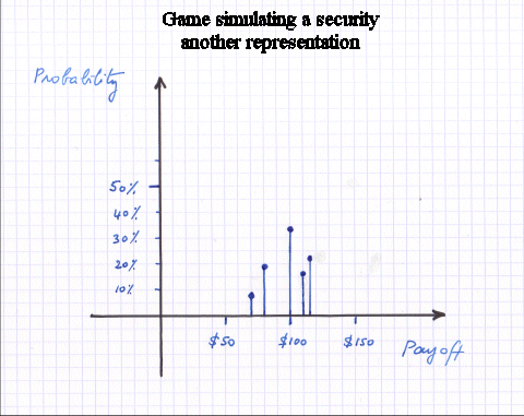
The usual representation of the possible values of X and their probabilities :

Some people find this representation of X, and its probabilities, more useful than the wheel shown previously. Some people prefer the wheel.
This graph is more customary.
We studied this little game because it is a good simple simulation of a real security. It is simpler, because :
When we become accustomed to the above kind of graph, we can readily see that the average value of X is in the vicinity of $100.
If we modify our wheel by introducing a new thin sector, with an angle of only one degree, and a payoff in this new sector of $1000 (and we reduce the $115 sector size from 80° to 79°) we will not change by very much the expectation of X.
The reason is that E(X) is a weighted average of the possible values of X, and the new value a6 = $1000 has a very small weight. The new value of E(X) is about $101. (This should come as no surprise since in the calculations we added a little less than $3 to the previous average.)
Indeed if we play the new game many many times, the outcome a6 will not come up very often. And therefore the average value of my outcomes will not change much.
Exercise : if we play the new game 256 times, what is the probability to never get a6 ?
Answer : about half of the time. (The experiment, here, is "play the new game 256 times".)
(The computation of the simple average of the possible outcomes a1 + a2 + a3 + a4 + a5 + a6 is subtantially modified by a6. It goes from 95 to 246. But it is of no concern to us.)
Becoming accustomed to financial calculations :
We will become accustomed to probability and financial calculations in the same manner we became accustomed to, for instance, debit and credit in Accounting. It took practice, just practice.
For instance : if we make a sale on credit, which account gets credited and which account gets debited ?
You have to remember this.
The different aspects of mastering a field :
Mastering a field of human knowledge, to guide human action, has four aspects
Last year we tried together to make elementary progress along these four aspects in the field of Accounting.
This year we will do the same in Finance. We begin with very simple stuff, but make sure we keep in sight the deep simple ideas. Little by little we will gather a culture, and also enter a bit into the technicalities of the discipline. Finally some of you may choose to go further into Finance and achieve some creativity.
In all fields of knowledge and action you will meet people (sometimes "eminent" people) who only master three or even two of the four aspects of their discipline, listed above.
Exercise :
Y is a random variable that can take the following values with the following probabilities :
| Possible outcomes ( ai's ) | Probabilities ( Pr{ Y = ai } ) |
| $45 | 20% |
| $80 | 35% |
| $250 | 30% |
| $300 | 10% |
What is the expectation of Y ?
(Ans : $142)