Finance with a review of accounting

Randomness of a security, risk-return graph, systematic risk and specific risk

The steps in probability theory

The presentation of probability theory requires several steps. If we miss no step it is reasonably easy to understand, and to use, but, if we miss a single step, it may become extremely confusing. So, here is a little review of the steps :

1. E : the experiment that produces a random variable X, and that can be reproduced (at least in theory).
2. X : the random variable. For each instance of the experiment E, X has an outcome x, which will vary from replication to replication of E.
3. X takes its outcomes in a set of possible outcomes :
   • the set of possible outcomes of X may be discrete and finite, in that case we denote it { a₁, a₂, a₃, ..., a_p }
   • or it may be the whole set of real numbers.
4. Replicating E n times will produce a series of outcomes of X : x₁, x₂, x₃, ..., x_n. Think of n = 1000 or 10 000...
5. Probability P : there is a measure of probability P attached to E . By this we mean that to any possible outcome of X, or range of values of X (if X is continuous), we can attach a probability :
   • if X is discrete and finite, for each possible outcome a_i, there is a number p_i = Pr { X = a_i }. The sum of the p_i's is 1.
   • if X is continuous, there is a density of probability f_X such that Pr { a ≤ X < b } = area beneath f_X between a and b.
6. Sometimes the p_i's (or f_X) are known to us, sometimes they are not. They are known to us, in particular, when the experiment E shows some symmetry, like a well balanced die, or spinning a well balanced wheel.
   • If we throw five well balanced dice, any outcome (a set of 5 integers, each between 1 and 6, and where the order matters) has the same probability : (1/6)⁵
   • If we spin a well balanced wheel, any angle A, measured in degrees, has the probability A/360 to be pointed at by the index fixed on the frame of the device. It is just a variation on the continuous distribution Uniform between 0 and 1.
7. When we don't know the p_i's, or f_X (and this is the case in real financial situations) , a sufficiently long past series of outcomes of X provides good estimates :
   • in a long past series x₁, x₂, x₃, ..., x_n, the proportion of x_i's equal to a₁ will be close to p₁,
   • or the proportion of x_i's falling between a and b will be close to Pr { a ≤ X < b }.
8. The fact stated in item 7 is basically a result in numbering. For instance, if we throw a coin 3 times, we are more likely to get different results (three fourth of the time), than three times the same result (one fourth of the time).
9. A numerical random variable X has (except in some mathematical situations which we are not concerned with in this course) a mean E(X) and a variance Var(X).
   • The mean (also called expectation) is the weighted average of its possible outcomes
   • It is also the value to which converges the simple average of a long series of outcomes
   • The variance is the expectation of the squared deviation of X around its mean
   • The standard deviation is simply the square root of the variance
   • The standard deviation of X is a measure of the variability of X around its mean.
10. Most continuous random variables we shall meet in this course will be normally distributed (bell shape density) with some mean m and some standard deviation s.

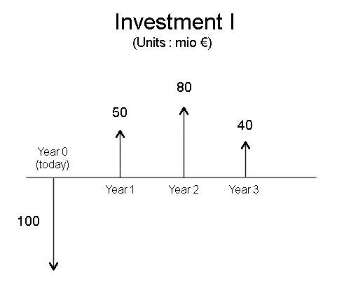
Probability theory as a toolbox for finance

With these elements of probability theory, we have tools to approach the study of investments (financial investments into securities, and physical investments into projects), which will produce unsure cash flows in the future. With the technique of discounting (which we will study in the next lesson) we will be able to attach a value today to future cash flows. We will be able to compare various investments.

We study essentially two situations :

• Investments into financial securities (stocks in the stock market) which will produce a cash flow one year later (for instance, by selling them back),
• Investments into physical projects, or financial securities (like bonds), which will produce a stream of cash flows over several years.

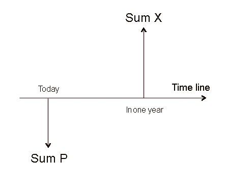
The two situations can be memorized with these two pictures :

Finally, we shall be concerned with profitabilities of securities. If we buy a security S today, for a price P, and S produces a cash flow X, in one year (and X is a random variable), then the profitability that we will make in one year is

R is a random variable, with possible outcomes, with a mean, with a variance and a standard deviation.

E(R) is denoted r. If need be, we use the more specific notation r_S. It is the expected profitability of the security S. Sometimes, for short, we call it, abusively, the profitability of S.

Standard deviation of R is denoted σ, or, if necessary, σ_S.

σ_S is, by definition, the risk of S. In other words, in finance, the risk of a security is the standard deviation of its profitability. Securities with zero risk are called risk free securities. At present, in the euro zone, they are sold with a discount of 2% on their future value. More risky securities are sold for less.

Exercise :

1. If we buy, today, one Google stock, for $312, and sell it in one year, do we know the profitability we will make ?
2. If we spend $1000 to buy a basket of securities (it is called a portfolio) reproducing more or less the Dow Jones Industrial Index, do we know how much money our portfolio will be worth in one year ?
3. Do we have past data to make a reasonable guess ?

We will extend the concept of profitability to a stream of future cash flows. For several cash flows, the usual notations are these :

initial investment : C₀ (akin to P in the case of one security)

future cash flows : C₁, C₂, C₃, ... , C_m, if there are m years. These extend the unique cash flow X of the one year case. And, like X, they are random variables. But, if we don't specify it otherwise, we shall directly consider the expectations of the future cash flows. And the C_i's will be expectations.

A slight difference between P and C₀ : usually, for a security S there is a market price today, that's what we call P. And we shall see how P can be computed. Most of the time, for a physical investment I which will produce a stream of future cash flows, there is no market price. But we have to invest C₀ to produce the stream of future cash flows. Sometimes it will be a good deal for us, sometimes it won't. This is what we shall study in the next few lectures.

Example of a security

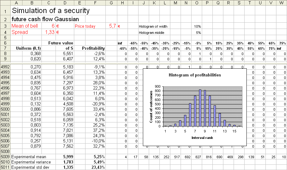
Consider a security S, with a present price P, and with a value in one year X. We shall work with a numerical example : assume X is normally distributed with mean E(X) = 6€ and standard deviation σ(X) = 1,33..€.

If P, the price we pay today for S, is 5,7€ then our profit will be X - 5,7, and our profitability will be (X-5,7)/5,7. Depending upon the outcome of X, we will actually make a profit or not. Our expected profitability will be E[ (X-5,7)/5,7 ] = E [ X/5,7 - 1 ] = E(X) / 5,7 - 1 = 5,26%.

Check with a simulation :

This Excel sheet presents the simulation of 5000 replications of the experiment producing the value of S in one year : we produced 5000 outcomes of X, and therefore 5000 outcomes of R = (X - 5,7)/5,7.

E(X) = 6, and the experimental mean is 5,999

σ(X) = 1,333 and the experimental std dev is 1,335.

E(R) = 5,26%, and the experimental mean is 5,25%

σ(R) = σ(X/5,7 - 1) = σ(X)/5,7 (because a translation of an RV does not change its std dev, and a rescaling rescales the std dev) = 23,39%, and the experimental std dev = 23,43%.

In order to understand finance, we must understand perfectly what this simulation does.

Suppose, now, that to purchase S, today, we pay a price P = 5€

With this price P, the expected profitability of S is 20% (= (6-5)/5). And the standard deviation of the profitability is 1,333/5 = 26,7%.

This can be checked again with a simulation. You are strongly encouraged to construct the simulation and check these figures by yourself.

Randomness of a security

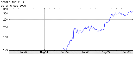
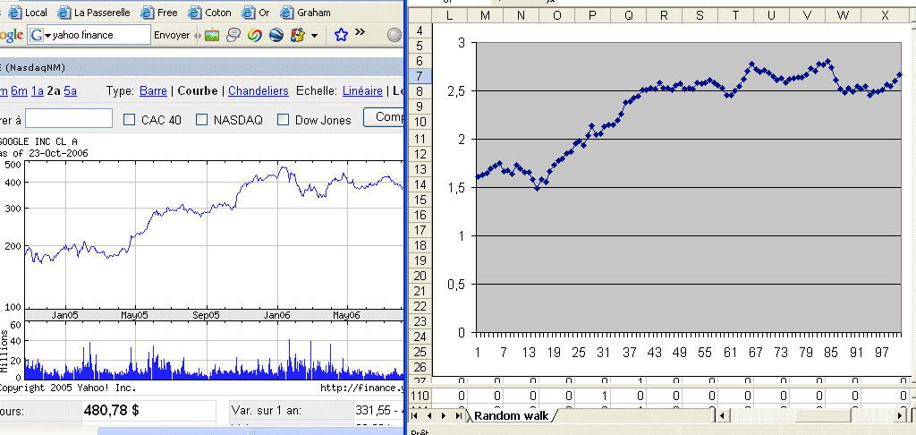
Let's consider a security S, with a price P today. Finance considers its value X in one year as a random variable. It will have an outcome x. This x will be the price of S in one year. Then S will have a value in two years, which is a random variable, etc.

The sequence of yearly prices is not a series of outcomes of one random variable, because they are related to each other.

Finance considers the series of profitabilities as a series of outcomes of one random variable, the random variable R. The series of prices is called a random walk. The multiplicative step to go from one year to the next is a random variable (1 + R).

In fact, if we look at Google prices over the last year we see readily that the prices are not outcomes of one random variable :

Random walks

The first scholar to talk about and study random walks in finance was Louis Bachelier, 1900. His doctoral work did not receive much consideration at the time, and he got his thesis with an average mark, and then went into obscure teaching positions.

Later on his work was rediscovered, in particular by Samuelson, in the early 50's, and became the object of much study. Today Bachelier is considered one of the towering figures of early modern finance.

He studied "arithmetic random walks", where one position differs from the previous one by an additive random factor D_n, with a steady normal distribution N(μ, σ). Then he refined his model to an infinitesimal additive component, leading to Brownian motion, and he got very close to the Black-Scholes formula of option theory.

Today, the preferred model for stock price evolution is the geometric random walk, where one position differs from the previous one by a multiplicative random factor (1 + R_n), where R_n has a steady normal distribution. A variant model considers that log(P_n+1 / P_n) is normally distributed.

In the previous section we have the representation, in a logarithmic vertical scale of the price of Google over time. A question is : is it reasonable to model it has a geometric random walk ? See next section for a discussion.

The three approaches to the variability of prices

There are three approaches to the study of the price evolution over time of a given stock.

1. The Modern Financial Theory (MFT), which is the classical theory of the present day, and is taught in business schools all over the world. It says that the geometric random walk model for the price evolution over time of a given stock is essentially a good one, and it proceeds to all sorts of calculations to optimize portfolios combining various stocks. The full-fledged theory of portfolio in MFT is called the Capital Asset Pricing Model (CAPM ; and in French MEDAF). We shall get a glimpse of it in the final lectures of the course

          Here is a comparison of Google prices and a computer generated geometric random walk (both with logarithmic vertical scales) :

          It looks like it makes sense to consider that Google prices follow a geometric random walk.

2. The chartist approach : chartists look at the past price curve and declare to be able to see "trends", "ceilings", "breathroughs through ceilings", "collapses", etc. and to make forecasts from these. For instance, when they have identified a breakthrough through a ceiling, they "know" that the stock price will jump substancially - not just a little - before the next downturn.
   

3. The Graham-Dodd approach, 1934, which says that even though in the very short run prices may be subject to variations well modelled with probabilities, it does not make sense to use probabilities to study price evolutions longer than a few months. Other more fundamental factors related to the operations of the firm and to its environment are at work, and must be identified to decide what is the "true value" of the firm. Then if the market, which according to this approach is often preposterous, is much lower, buy. And if it is much higher, and you own stocks of the firm, sell. This approach relies on the concept of "true value" of the firm, coming from various Discounted Cash Flow analyses of its future earnings (see lesson 8). Warren Buffett was a student of Graham, has applied his principles all his life, and became one of the richest men on Earth. As Mark Rubinstein says (a proponent of the MFT), it is difficult to argue against success.

The risk return graph

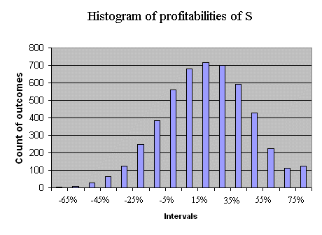
When considering securities traded in the stock market (shares of firms) we will often use the so-called risk return graph : on a graph with axes risk and return, we will position the various securities under study. For instance, let's position the security S with price P = 5€, and a normally distributed payoff X, with E(X) = 6€ and σ(X) = 1,333€.

We can compute E(R_S) and σ(R_S), but let's take the opportunity of this operation to read these two quantities from a histogram obtained from a large simulation. The profitability of S has the following histogram (produced with 5000 outcomes of R_S) :

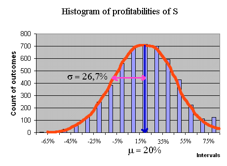
We can read from this graph E(R_S) and σ(R_S) :

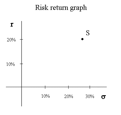
And now we can position S on the risk return graph, like this :

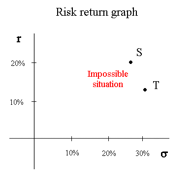
Systematic risk and specific risk

We have already briefly mentioned that stocks, in the stock market, have a systematic risk (fundamentally linked to the randomness of the economy) and a specific risk (akin to an extra random quantity added to their future cash flow, with mean zero, and that would be produced by the equivalent of a random generating device).

Investors are risk averse concerning systematic risk. They don't care about specific risk because there are ways to eliminate it (more on this later in the course).

Consider two securities, S and T, with different systematic risk and no specific risk. Then, if both promise the same expected cash flow in one year, investors will pay less for the riskier one. As a consequence, the riskier one will have a higher expected profitability.

This has a consequence on the risk-return graph : if we look only at securities with systematic risk, and no specific risk, It is not possible to have two securities S and T positioned like this :

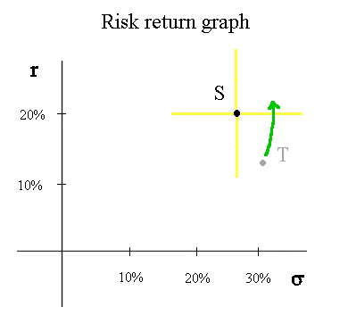
Indeed, if S is a security available in the market with r = 20% and σ = 26,7%, nobody will buy another security T, with less profitability and more systematic risk. So the price of T will decline until its profitability becomes higher than that of S. The point representing T will move to the top and slightly to the right :

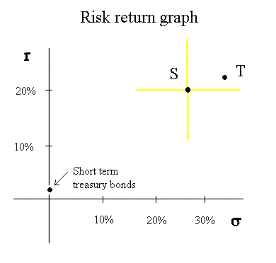
Finally, let's mention and position the risk free security : the short term Treasury bonds (yielding, at present, in Europe, 2%) :

Go to lesson 8