Wednesday October 13th 2004

Finance : first lecture (part two).

Review of the first part of the lesson
The second part of this lecture is devoted to computing the right price of securities
Suppose a security S promises to pay me $100 in one year. How much should I pay to buy S today ? (Is $80 a good price ?)
Let's look at a higher price P. If we pay $99 for the security S, is it still a good price ? (Ans. : No. We can make a better investment with government bonds.)
A little bit of geometry to explain 1/(1 + ε) ≈ 1 - ε
Recap so far
US Treasury rates since 1990
Investments the outcome of which is not sure
Risky securities
Concept of random variable
Definition of a random variable
Formalisation of a random variable
Examples of random variables
     A process manufactures light bulbs
     Random variables related to throwing dice
     Measure the temperature in the yard at noon
Simulating random variables with a computer
Summing up two dice
Summing up the results of 5 throws of a die (a bell curve taking shape)
When we sum up many RV, the result (which is also random) has a distribution of probability of outcomes which is a bell shape curve
A very nice simulation with little balls falling through a mesh of nails
Experimental probabilities
Do not to mix up the long series of outcomes x_i's with the small set of possible outcomes a_i's
Study of two securities S and T, one of them with no risk and one of them with risk
How much should we be willing to pay for T ?
The two attitudes toward the risk represented by the variability of T
Gamblers are not stupid, but they are not investors
Random variables in Finance

Review of the first part of the lesson

You will have to review the first part of the session carefully to make sure you understand it well. This is necessary to get this finance course on a good start. It was rather substantial but, I believe, reasonably simple. I covered a lot of ground and I will still cover a lot of ground in this second part.

Let us check quickly what we learned in the first part of this session :

- Money and value: in the casual use we make a them, we understand them very well.

- Accounting: we spent a whole year together learning that.

- Assets: it is a part of accounting.

- Money: it is this paradoxical asset that is very liquid and very useful to pay, and yet that we do not want to keep as is, because it does not produce value by itself. It doesn't "work". It does not fulfill the purpose of finance which is "how to transform the value I have into more value?"

- We saw two types of investments: investments into physical projects ; and also investments that are indirectly investments into projects, that is investments into securities. These financial investments are fine investments as well.

- I was able to formalize a bit more : finance looks at the variation of value over time and takes into account in some way, that we shall presently study, the risk.

- Then I talked a lot about interest rates, in particular risk-free interest rates, government borrowings, the story of interest rates in the United States over the last two centuries.

- I tried to relate all these concepts to the world economy, and to the big concrete questions it poses concerning the well-being of humankind on this planet.

The second part of this lecture is devoted to computing the right price of securities,
- first of all when there is no risk
- and then when there is risk,
and the tool to work with risk, namely probabilities.

To start easy consider a security, that is a piece of paper promising some value in the future (that's what a security is). Let's call it S.

Suppose S promises to pay me $100 in one year. How much should I pay to buy S today ?

Which price P ?

It is, viewed in a reversed way, the same question as the interest rate we looked at before. But instead of knowing the value we pay today and discussing how much we should get in the future, we start from the sum of money we shall receive in the future and we look at the price we should pay today.

So, someone offers us to sell us a security S, that is - as we saw - that person wants to borrow money from us. The security we are offered promises to pay us $100 in one year. How much should we pay for it today ?

If we pay today $80, is it a good deal for us ? Is it a good price (for us) ?

Answer: Yes it is a good price ! We pay today $80, and in one year we get $100, we make a 25% profit over one year, it is a good deal for us !

Caveat : It is a good deal provided we are sure that we shall get these $100 in one year... That is, provided the borrower is a trustworthy person.

Let's look at a higher price P. If we pay $99 for the security S, is it still a good price ?

Answer: No. It is no longer a good price.

The reason is somewhat technical. If we pay a price P = $99 today for S, and receive a sum X = $100 in one year. We will make a profit R (computed in percentages) of

But we can get a better profit by just investing our money in US Treasury bonds. Remember US Treasury bonds, as of October 2004, yield 1.75%. If we invest our $99 in US TB we will get, in one year, $100 and 73 cents. That is better than $100.

If we write 1.75 = r₀ , the risk-free interest rate paid for safe borrowings in dollars today, we see that we want to pay no more than a price P such that

( 100 - P ) / P =  r₀  [equation 1]

that is, P = $98.28.

Any price above this figure is too high for us. Any price below $98.28 is, of course, fine for us, but it is not for the borrower: the borrower wants to receive $98.28 today, in exchange for a payment in one year of $100.

So P = $98.28 is the right price, considering today's value of  r₀ .

Equation 1 is often rewritten into the following equivalent Equation 2 :

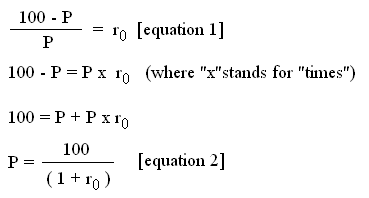
These two equations (equation 1 and equation 2) are equivalent. It is quite important that you become very familiar with both.

The correct price P to pay today for the security S (that promises to pay $100 in one year) was computed using equation 2 into which we plug the correct risk-free rate r₀

correct price P for S = $100 / ( 1 + 1.75% ) = $98 and 28 cents.

To relax : a little bit of geometry :

(you need the police "symbol" installed on your computer to view correctly Greek letters)

In Finance we shall make a great use of equation 2, and usually the interest rate r we will plug (where we put r₀ ) will be reasonably small. So we will often use the following mathematical fact :

(where ε, pronounced "epsilon", stands for "a small quantity" ; and  ≈ stands for "is almost equal to")

Why is that ?

There is a nice simple geometric explanation, that helps remember it :

- look at a square of size 1 x 1

- then look at a rectangle of size  (1 - ε)  x (1 + ε)

The surfaces of these two figures differ only by a very small element, a small square of size ε x ε (also noted ε² )

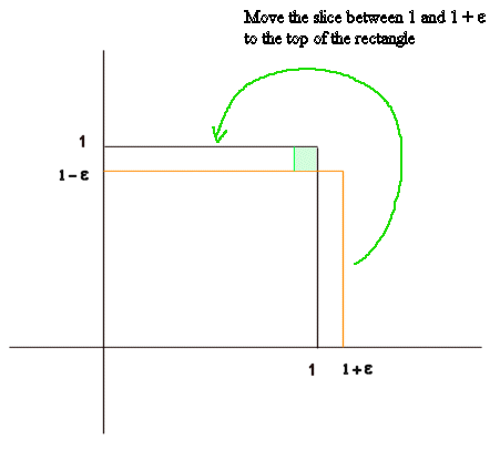
Indeed we see that the surface of the rectangle (1 - ε)  x (1 + ε) (with orange sides), if we move the right slice to its top, corresponds to the surface of the square 1 x 1, but for a the small blue square (which has the size ε x ε ).

Applications :

1 / 1.01  ≈ 0.99

1 / 1.0175 ≈ 0.9825

It even works for a larger r :

1 / 1.2 ≈ 0.8  In fact the exact calculation is 1 / 1.2 = 0.8333...

Recap so far :

If we lend $100 to a risk free borrower (for instance the US government), in one year we get back $101.75.

Or entirely equivalently if a risk free borrower sells us a security S (in dollars), that is borrows some dollars from us, and the security promises to pay us back $100 in one year, we should pay today $98.28 for it. In other words, we should lend $98.28 to the borrower.

These calculations, at first, require a little bit of mental gymnastics. They are not complicated at all, but before they become natural to us we have to practice, and practice again. It is a bit like "credit" and "debit" in Accounting : at first it does not come naturally to the mind, it requires a lot of practice, and then it becomes a second nature to know whether a recording is a debit or a credit.

We will practice a lot with equation 1 and equation 2 !

If we purchase the security S at a lower price than its normal price, we can actually make money right away ! Indeed, suppose that for the security S (promising $100 for sure in one year) we pay today only $90 to our borrower. Since this security will bring $100 in one year, there are plenty of people in the market willing to buy it for $98.28, so we can sell it back right away, and instantaneously earn $8.28.

In textbooks that were written some years ago, the risk free rate r₀ is way higher than 1.75%. Usually it is between 5% and 10%, because that's around where the risk free rate moved in the mid 90's (source : http://www.1loansusa.com/treasuryrates/1990-1999.html ).

US Treasury rates since 1990 :

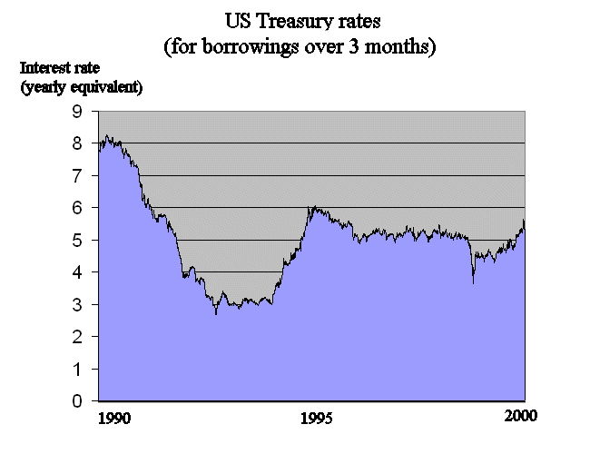
For instance, if we take r₀ = 6% the price of a security S promising for sure $100 in one year is

it is not far from 94% as we know it must be.

So far we considered only sure borrowers ; borrowers that are entirely trustworthy ; deals where we are sure that the contract will be settled according to plan.

Of course in Finance we shall also deal with investments the outcome of which is not sure.

In fact investments where the future money we shall get back is a sure figure are quite the exception, they concern only borrowings by large governments of prosperous countries, and borrowings made in their money of course. They relate to the deep meaning of money, concepts that we shall not study in this finance course.

Investments the outcome of which is not sure :

When we invest money into a physical project, for example a new machine to expand our production and our sales, we are not sure that it will be a success. It is uncertain, that is we don't know for sure whether we will get our value back and more. Many circumstances can make the investment perform less well than planned: the market may change in the meantime, competitors may come up with a better product than ours, we may encounter difficulties running the new machine, etc.

Same is true with financial investments. A financial investment, the purchase of a bond, or of a stock in the stock market, is an expenditure of money today in order to get more money in the future (either via interests or dividends, or via capital gains, or both). But there again, with the exception of short term government borrowings, we are not sure of the money we shall get back in the future. There is a risk.

For a stock, for instance, everybody is familiar with the fact that we don't know for how much we will be able to sell it back in one year on the stock market. Next year prices are uncertain. In the newspaper we can look at prices today, and also at historical prices. But we cannot look at next year price (like we actually do for short term risk free government borrowings!).

Concerning the future, in the newspapers, we can only read what financial analysts think. (It's interesting, sometimes...)

Risky securities

We shall call it S again. What do we mean by a risky security ?

In a simplified description it means this: today, for the security S, I pay a price P, and in one year I'll get back a sum of money X, the actual amount of which is not a sure figure.

In a simplified version of life, this is a correct model for a physical investment, as well as for a financial investment (with the exception of investments in short term government bonds).

The cash flow X that we will receive in one year is a random variable.

It is no longer a fixed number. So we will have to study in detail what we mean by a random variable.

Concept of random variable

Random variables will be the topic of the rest of this lecture.

Random variables are a concept we did not study in high school. Yet we are familiar with randomness in our everyday life, perhaps without having a clear description for it.

I'll explain this new concept. New concepts are always, at first, vague. This is normal. That's the way we learned all the concepts we have in our mind: at first they were vague.

We absorbed many many new concepts when we were toddlers. Now they are so clear to us that we tend to forget that at some point they were quite surprising. And before we constructed models in our head, some phenomena, that today we know are impossible, did not surprise us. For instance this: I put this red marker in my right pocket and... here I pull it off my left pocket :-)

We know this is impossible - there must be a trick - because we modeled a long time ago certain perceptions as "objects" that move but stay the same objects. And they don't disappear in one place to reappear in another one.

Not every being understands this: take the sea lion that we watch at the circus playing with a yellow ball ; you throw the ball behind a sofa, and it rolls and then reappears on the other side ; the sea lion sees a new ball ; it doesn't figure out in its mind that it is the same ball.

We are capable of constructing mental representations of fixed objects, even when some characteristics of these objects change, for instance their positions. Don't be mistaken, it took a mental effort to do this. The question even interested philosophers in the XVIIIth century: if a piece of wax can change shape, color, position, become liquid, or gas, etc. what remains "the same" in these manipulations ? (At the time they did not have the atomic theory to help. And beware, the atomic theory is full of models quite opposite to common sense. For instance having one photon pass at the same time through two holes and, on the other side, create interferences on a screen. Don't mix up "reality" (that is, as far as we can say, raw "perceptions") and the representations of it we work with...)

In fact we are also familiar with concepts that, if we think of them, are still quite unbelievable: we are told, contrary to evidence, that the Earth is not flat with an "up" direction and a "down" direction, but a sphere floating in space in the Universe, and nobody falls...

(A blurb on Christopher Columbus who thought he had proved the Earth is round even though he only went to America, and Magellan who tried again but died in the Philippines...)

(A blurb on particles that take 8 minutes to come from the Sun, and yet whose life lasts a fraction of a second...)

OK, so we see, in particular, that, perhaps without realizing, we are quite accustomed to "entities" that we consider "to be staying the same" and yet many characteristics of which change all the time. This will be an aspect of random variables.

A random variable is "an entity" that I can produce several times, and that each time has a different actual "outcome" and measure.

The setting to produce the outcomes of the random variable is called "the experiment". It is quite important to describe exactly which experiment we talk about when we talk about a random variable.

Definition of random variables :

There are some physical situations where an entity can be observed (and measured), the situation can be reproduced, and the actual measurement (often a number) changes from replication to replication of the situation.

The "entity" is not defined by its measurements. The measurements change, the "entity" does not. We call the "entity" "a random variable", each instance that can be observed and measured "an outcome of the random variable", and the physical situation that can be reproduced "the experiment".

There is no concept of random variable without an experiment, in which the random variable is observed. And the experiment can be reproduced, at least in theory.

Formalisation of a random variable

For those of you who want to begin a deeper study of probability and random variables, here are some introductory explanations about the concepts and notations ordinarily used :

Each outcome of the experiment E is considered as producing an elementary event ω, out of a whole set of possible ω's. The set of possible ω's is denoted Ω. It is called the "universe" corresponding to the experiment E. An "event" A in the universe Ω is a subset of Ω. (It is therefore made of a collection of elementary events.)

Attached to the experiment E and its universe Ω there is a probability distribution P, which to any event A gives its probability : it is a measure between 0 and 1. For instance, for certain events, it will be possible to write P{A} = 75%.

A random variable X (if it is a numerical one) is a function from Ω to the set of real numbers R. To any outcome w in Ω there corresponds a value of X, denoted x = X(ω), which is also called "an outcome of X".

The possible values of X are a subset of R or the whole of R. We can define events in W with reference to values taken by X, for instance if X is a random value in dollars, {X ≤ $30}is an event in Ω, and we can talk about P{X ≤ $30}, which is a number between 0 and 1.

Examples :

1) A process manufactures light bulbs, as identical as we can make them. Pick one light bulb in the bin at the end of the machine, and measure its lifetime (or something quicker, but linked to its lifetime). We will get a figure around 50 000 hours. But each time we take a new light bulb, produced by the same process, even the same machine, we shall get a different figure. For instance we may get the following series :

These six numbers are six outcomes of our random variable.

The next day we may decide to work again on the same experiment and the same random variable. We shall not get the same series of numbers, and yet we will be working on the same random variable. So we should not mix up the random variable and one series of outcomes of it.

Don't forget : when we talk about a random variable, we have to be extremely precise which experiment we are talking about.

For example, if I say "select a person at random, what is the probability this person is Chinese ?" Well the description of the experiment is not precise enough.

 Is it worldwide, with everybody having the same chance to be picked ? In this case the probability is about 1/4.

Or is it in this classroom, with everyone having the same chance to be picked ? In this case the probability is much higher.

2) It is customary to mention random variables related to throwing a die. Let's abide by the custom.

2a) Let's throw a die once. That's "the experiment". And the "random variable X" is "the face showing up".

Possible outcomes of X : 1, 2, 3, 4, 5 and 6.

Each outcome has the same probability : 1/6. That is about 17%.

Outcomes of random variables don't have to be numbers. It can be colors of socks picked from a drawer, sexes of creatures, etc. But in Finance the RV we shall encounter will take numerical values.

2b) Let's throw 2 dice. This is a different experiment from above.

What is the probability that no die shows a 4 ?

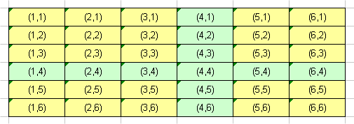
You may list all the possible pairs. There are 36 possible pairs (where we clearly distinguish die one, from die two. The pair (2,5) is not the same as the pair (5,2).) Each pair has the same probability. You can count (or calculate) that 11 pairs have one or several 4.

So Probability {we get no 4 in any of the two dice}= 25/36

Those of you who like calculations will see that it is 5²/6² because it is the number of cells with no 4 in the following array (the yellow ones) divided by the total number of cells.

Exercises :

1) we throw a die four times. The probability to get no 2 is more or less than 50% ?

(Answer : slightly less.)

2) we throw a die 16 times. How likely it is we get no 5 ?

(Answer : about 5% of the time.)

3) Third example : the experiment is "Measure the temperature in the yard at noon".

What is the probability to get more than 20° Celsius ?

Again, we have to be more precise about the experiment we have in mind. Do we mean to measure the temperature any day "picked at random" ? Or do we mean to measure the temperature any 13th of October ? It is definitely not the same experiment ! And the random variable would not be the same, and would behave differently.

For instance if the experiment is "Measure the temperature in the yard any 13th of October" we know that the probability we get 20° or more, like we do today, is small. Today is an unusually hot day for the season...

Note that "Measure the temperature at noon, any day" is not a very interesting experiment, because we know that the temperature depends highly upon the date.

When we study a random variable we want to eliminate all the factors that we know will influence the outcome.

Simulating random variables with a computer :

Computers are very useful to study random variables and particularly to get a feel for them.

I can generate with a computer the throws of a die. Here is a nice website that does it : http://www.stat.sc.edu/~west/javahtml/CLT.html

If I throw a die 10 000 times and I count how many times I got 1, how many times I got 2, how many times I got etc. up to face number 6, I can represent these 6 proportions from my actual big experiment (throw a die 10 000 times). We know from our daily life experience that these 6 proportions will be close to 1/6 each.

With a computer we can simulate in a second this big experiment instead of painstakingly carrying it out with a real die. Here is one result :

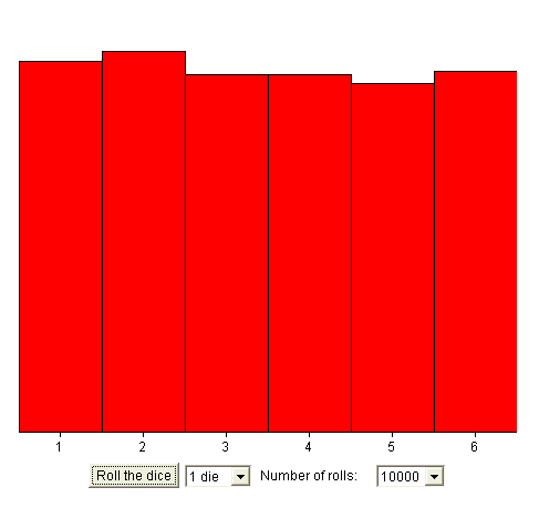
If we do it again we won't get exactly the same histogram, but once again it will be close to evenly distributed.

The simulation applet is very nice to investigate the behavior of random variables.

Summing up two dice :

For instance, consider the experiment E : "throw two dice". The random variable we want to study is

X = sum of the two dice

Let's repeat the experiment E 10 000 times. And let's see what is the distribution of the outcomes of X.

We know that the possible values of X are 2, 3, 4, ..., 11, 12.

Here is an experimental distribution :

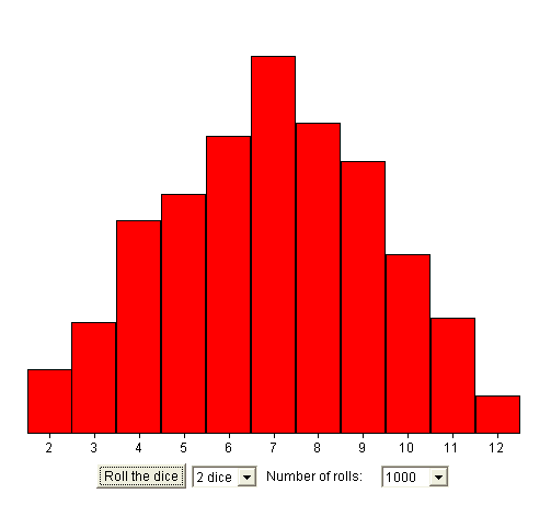
Not quite exactly a triangle (we got more 2's than 12's) but almost. In fact it is easy to figure out (from counting) that the theoretical probabilities form a triangle.

Now more surprising.

Summing up the results of 5 throws of a die :

Now the experiment is "throw a die 5 times" (or equivalently "throw five dice"), and the RV we are interested in is still the sum of the results of the five throws.

X can take the values : 5, 6, 7, 8, ... ... , 28, 29, 30.

The shape of the experimental distribution of outcomes of X if we carry out the experiment 10 000 times may come as a surprise :

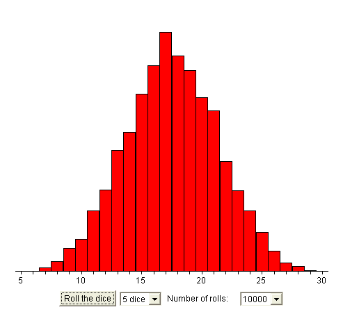
A curve that approximates a bell !

(Remember: if we carry out another batch of 10 000 replications of the experiment we will get a slightly different curve, but with the same general shape.)

In fact this is an important result in probability theory (it was discovered by the great German mathematician Gauss (1777, 1855)). It has a more general form than what we just saw :

when we sum up many RV the result (which is also random) has a distribution of probability of outcomes which is a bell shape curve.

It is also called a Gaussian curve. There are many Gaussian curves, with different centers (in the picture above, the center is between 17 and 18) and different narrowness.

It is because random variables in Finance are often the result of many more or less additive random effects that Gaussian distributions are the most frequent distributions we will encounter.

Exercise : practice a lot by yourself with the applets of the site http://www.stat.sc.edu/~west/javahtml/CLT.html.

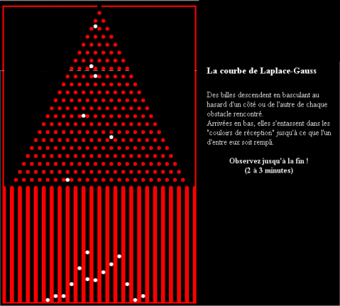
Take a look too at this fine simulation of small balls falling through a mesh of nails : http://rigolmath.free.fr/gauss/iegauss.htm

Experimental probabilities :

Because we all know this fact from experience, I've used above, without making a special mention of it, the following result :

when the possible outcomes of a random variable X are a₁, a₂, a₃, ... a_p ,

with probabilities Pr{X = a₁} = p₁,    P{X = a₂} = p₂,  ...   P{X = a_p} = p_p ,

even if we don't know the actual exact p_i's we can estimate them by repeating the experiment in which we measure X many many times.

For instance, suppose I've repeated the experiment 10 000 times, and measured, therefore, 10 000 outcomes of X, I got a series of 10 000 numbers. It is customary to note them

x₁,  x₂,  x₃,  x₄,  ...  ...  ...  x₁₀₀₀₀

IMPORTANT : Do not to mix up the x_i's with the a_i's_.

Each x_i is a number among the a_i's. We may have only three a_i's (i = 1 to 3), and 10 000 x_i's.

For example, in the experiment which is "throw one die", and X which is "the number on the face up", there are six a_i's ; they are 1, 2, 3, 4, 5 and 6.

If we throw the die 10 000 times, we shall get a sequence (or series) of 10 000 outcomes, x_i's, each of them is a number among 1 to 6.

For any random variable (technically: for any discrete RV) in order to estimate, say, p₃ (the probability that X take the value a₃) the most usual way is to count how many of the outcomes x_i's were equal to a_{3 ,} and divide by 10 000. We know that the result (the estimation of Pr{X = a₃}) will be close to the actual p₃.

We need to introduce one last concept today: the attitude of finance people toward risk.

Study of two securities S and T, one of them with no risk and one of them with risk:

Suppose we have two securities S and T.

Suppose S has no risk : it is a promise for a sure well specified sum of money M in one year. And T has risk, that is the amount of money X it promises to pay in one year is a random variable.

Aside from that S and T are somewhat comparable, in the following sense :

The average value of X is M, the same amount of money S promises with no uncertainty.

For instance M is $110.

So in one year S promises to pay for sure $110. We know that the price of S today is 110 / (1 + 1.75%) = $108 and 11 cents.

T is different. It is a realistic security (that is not a Treasury bond). The amount of money it will pay next year is not a sure number. But for some reason (for instance, from past study) we know that its average value is $110.

In a series of replications of the experiment producing the payment X of T in one year, we may get, for instance, the following numbers :

These outcomes are only to help understand. Next year T will pay one figure (an unknown figure, but only one).

How much should we be willing to pay for T ?

This is a big question.

On average, T will pay exactly the same amount as S, namely $110.

It may even pay more. And it may pay less.

The two attitudes toward the risk represented by the variability of T :

There are basically two attitudes toward the risk represented by T :
- some people will prefer S to T, "because S is surer",
- some people will prefer T to S, "because that's the only way to gain possibly even more than $110, and anyway it has the same average value as S"

Finance people prefer S. For T they will offer a price lower than for S. For S we saw that they offer $108.11 .We shall see which price financiers are willing to offer for T. And it will be its price actually seen on financial markets.

Those people who prefer T are gamblers.

There is no way to demonstrate that one category is right and the other wrong.

(On the other hand, there are farfetched ways to demonstrate that gamblers actually behave like financiers.)

Gamblers :

Gamblers are attracted by risk, and by small possibilities to earn large amounts of money ; so much so, that they are even willing to buy for a substantial price promises which will pay an average value much less than the price they pay.

This is the case of lottery players. They regularly buy for, say, $10 a ticket that will earn them $5000000 with probability 1/1000000, and will earn them $0 with probability 1 - 1/1000000.

The average money they will get is $5.

To pay $10 for such a ticket is nonsense for a financier. Not for a gambler.

States use the fact that many people are gamblers and organize lotteries. Lotteries bring so much money to states that in most countries only state organized lotteries are allowed.

Random variables in Finance :

In Finance we make an important use of random variables because that's the best way that was found to handle the uncertainty inherent to investments.

In this first course, we will use only simple characteristics and properties of random variables : their average value, and their dispersion around their average value (also called their "spread") and a few other things. The random variables we will work with will be numerical ; they will take dollar values, or euro values. Or they will be percentages (for instance : profitability).

go to lecture 2