(écrit en octobre 2004)
Calculus is one of the great achievements of human thought. Its history illustrates the slow progression from Realist thinking to Nominalist thinking and the tremendous power of the latter approach to solve problems. The description of the use of calculus in probability theory is the occasion of a brief survey of this evolution of human thoughts.
- The problem we have to get around concerning continuous random variables
- Cumulative distribution of probability
- The slope of F and the density of probability f
- Tangents and surfaces
- The fundamental result of Calculus
- Usefulness of the fundamental result of Calculus
- Primitives
- The surface area S(x) between 0 and x under a function f is a primitive of f
- Computers and primitives
- Leibniz notations
- The genius of Oresme
- Great ideas and technical developments
- Mathematical models
- Calculus and probability
The problem we have to get around, concerning continuous random variables :
Back to some theory.
Even though continuous random variables have outcomes, just like discrete RV, the set of possible outcomes is now infinite and continuous, and the probability of each specific outcome is zero.
If we have a portfolio of securities and we call X its profitability in one year, the probability that X be any precise figure is zero :
Pr{X = 72.32653746...%} = 0
In order to get around this problem we shall introduce the concept of density of probability in the vicinity of any possible outcome of X.
This pertains to the field of Calculus.
We shall not use Calculus in this Finance course, so we can relax and take a look, if we like, at the next sections just for our culture. I will try to make them as simple as possible. And I will introduce some historical notes to give them more life.
Study becomes mandatory again only when we reach the section concerned with histograms.
Cumulative distribution of probability :
For any random variable X, taking values in the whole range of numbers from - ∞ to + ∞, we define the function F as follows :
for any possible outcome x,
F(x) = Pr{ X ≤ x }
It is called the cumulative distribution of probability of X.
This function is defined even for discrete numerical random variables. For instance, for our wheel with sectors,
F($100) = 61.1%
because it is equal to Pr{ X = $70 } + Pr{ X = $80 } + Pr{ X = $100 }.
But for discrete numerical RV the cumulative distribution of probability is not a very interesting function.
On the contrary, for continuous random variables F(x) is very useful.
F is a function that increases from 0 to 1, since it represents increasing probabilities.
For the random variables we will meet in this course, the cumulative distributions of probability will always be nice smooth functions.
Here is an example of graph of a cumulative distribution of probability F :
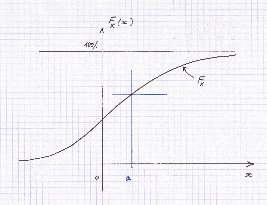
For any point "a" on the abscissa, F has a value F(a).
René Descartes (1596-1650) is usually credited with being the first mathematician to have invented such a representation of a function.
But in fact the idea is already very clearly expressed in the work of Nicolas Oresme (born in 1322 or 1323, died in 1382), almost three centuries before : (stated in modern language) "when a quantitiy y is a function of another quantity x, if we display all the x values along a horizontal axis, and for each x we raise vertically a point above x at a height y, we get a very interesting curve : it somehow represents the relationship between the y's and the x's".
Nowadays we just call this curve "the graph of the function".
The slope of F and the density of probability f :
Except for teratologic random variables that don't concern us in the course, the function F is nice and smooth.
At any point [a , F(a)] there is tangent straight line to F (in red in the graph below)..
We shall be very interested in the slope of this tangent straight line. This slope at "a" is also called "the rate of variation of F at a".
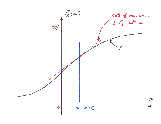
On this graph, for instance, at the point [a , F(a)], the slope of the tangent is about 0.7.
This means that if "a" moves to a point "a + e" close by, F(a) moves to a value F(a + e ) ≈ F(a) + 0.7 times e.
Here is a magnified view of what happens around the point [a , F(a)] :
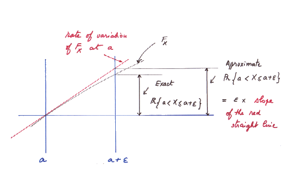
The rate of variation of F at the point [a , F(a)] is denoted f(a). The precise definition of the function f is
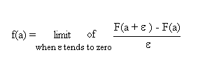
This function f is also called "the derivative of F".
The interesting point about it is that f is the density of probability of X around the value of the outcome "a".
Indeed
Pr { a < X ≤ a + e } ≈ e time f(a)
This is exactly the definition of a density. In fact we are all quite familiar with the concept of density. For those of you who like Physics, remember that a pressure can be viewed as a density of force at a given point. The notion of density is useful because, when considering, for instance, the pressure on the wall of a vessel, the forces vary from area to area (for instance from top to bottom), and the force at any "punctual" point is zero, so a concept of density is useful. This is the role of pressure in Physics.
The notions of density, intensity, pressure, slope, etc. are all the same : a quantity divided by the size of a small vicinity, which gives a local rate of the quantity. Examples : salary per hour, slope of a trail, pressure on a surface, flow of water in a tube per unit of time, mass per volume, speed, even variation of speed over time, etc.
The inverse process, going from rates to a global quantity, i.e. multiplying a rate by the size of a small vicinity to obtain a quantity over a small vicinity, and summing this up over many small vicinities to obtain a global quantity, like going from a density of probability function to the probability of X falling into a segment a to b, will also be of interest to us.
So, for a continuous random variable X we shall be concerned with its density of probability at any possible outcome a , because the concept of Pr{ X = a }, that we used for discrete random variables, has become useless (it is always zero).
Here is the graph of f for X (also called its "frequency distribution") :
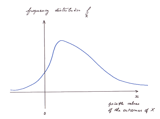
We are now in a position to point out the nice relationship between tangents and surfaces :
- We saw that f(a) is the slope of the tangent to F at the point [a , F(a)].
- We saw that Pr{ a < X ≤ a + e } ≈ e times f(a).
- This is almost exactly the surface of a small vertical slice under the curve of f, between "a" and "a + e".
- This is also the difference between F(a + e) and F(a)
- So for a larger interval a to b, the surface under the curve of f is F(b) - F(a).
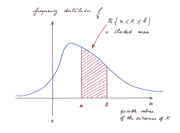
This is the fundamental result of Calculus :
for any nice and smooth function F, if we denote its derivative f (that is the slope of the tangent of F at any point), then the area under f between a and b is F(b) minus F(a).
In other words, and more loosely speaking, the operation of determining a tangent and the operation of determining an area are inverse operations.
Secondly, if two functions F1 and F2 have the same derivative f, they must be either equal or differ by a fixed constant.
We can readily see this because the function F2 - F1 has everywhere a tangent that is horizontal.
| We can state in another more punchy way the fundamental
result of Calculus : The rate of variation of the surface area S(x) under a curve f, between 0 and x, is precisely f(x). And, surprisingly enough, this result often lends itself to an easy calculation of the numerical value of S(x). (Illustration in the next section.) |
This nice result escaped ancient Greek mathematicians.
They were only able to compute areas of simple geometric figures. For more complicated figures they usually were not able to compute areas.
Why did not they realize the deep and nice link between tangents and surfaces ? Probably because most of them were profound Realists. Plato, with his ideas about the cave and the shadows, believed in a "true reality", and therefore in a unique form. They could not conceive that some variable quantity could at the same time be represented as a surface area and as a curve. It took the freedom of abstraction of the Nominalists of the late Middle-Ages to shatter this wall.
It was not until Newton and Leibniz (XVIIth century) that the link was definitely elucidated and Calculus could be launched. But this link was already clearly understood by Oresme (XIVth century).
Every great idea is built upon previous great ideas.
Greek mathematicians were great at the geometry of simple figures in the plane, for instance triangles about which they knew just about everything, with the exception of Morley result, discovered only in 1899 ! (Take any triangle, cut each angle with lines into three equal parts, the six lines intersections form an equilateral triangle. In fact Morley result has a deep meaning as regards the links between geometry and algebra : Alain Connes's proof of Morley's result, published in 1998.)
And precisely, Greek mathematicians did not use algebra. It is the arabic word al jabr, introduced for the first time by author al-Khwarizmi, in his book "Kitab al-Jabr". Al-Khwarizmi (780-850), whose name gave "algorithm", lived in Baghdad in the early IXth century.
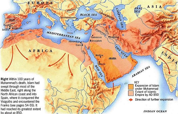
Illustration source: http://www.silk-road.com/maps/images/Arabmap.jpg
Because Greek mathematicians did not use algebra, they could not reach the more free attitude toward mathematical concepts necessary to invent Calculus. Greek mathematicians accepted to consider ideal figures (like the triangle) but required that they looked like things they readily saw with their eyes. They did not realize that "what they readily saw with their eyes" was just the result of mental constructions every human being carries out in his early youth, and that those are to an extent arbitrary as long as they model efficiently what we perceive.
Simply stated : Geometry does not come from perceptions ; it is the other way around. Our perceptions, as we think of them in our mind, result from the organizing process we apply to them with the help of usual 3D geometry. This question was already addressed by Kant, and other philosophers. No definitive answer was ever offered (which is, customarily, the mark that the whole framework within which the question is posed ought to be revamped). The most profound answer, in our opinion, is that of Wittgenstein in his "Tractatus logico philosophicus" (who declared : "Wovon man nicht sprechen kann, darüber muß man schweigen").
Since we are all alike we build more or less the same conceptions (this is true only for the simpler shared ideas, not for more personal views). Maria Montessori (1870 - 1952) understood this, and it lead her to recommanding new ways of organizing kindergartens and educating babies. Some of her ideas every nanny knows who gives her set of keys to the baby to play. It also lead to modern Fisher-Price toys, which are different from those available in 1900. (The next generation of toys will be even more remote from a "representation of reality" because it is unnecessary, misleading and mistaken.)
The more free attitude necessary to make progress was reached little by little by certain thinkers of the Middle-Ages (not all of them), after a large mix of cultures coming from the late Greeks, the Indians, the Sassanids, the Arabs, and some others, took place in the Old world, between years 0 and 1000.
This map offers a breathtaking view of the evolution of civilizations between -1000bc and now. (Time in abscissa, and, more or less, Regions of the Wold along the ordinate axis. From bottom up it corresponds- with the exception of Egypt - to East to West, which is the general movement of populations, in historical times, on Earth.) :
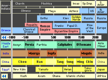
Source : http://www.hyperhistory.com/online_n2/History_n2/a.html
All this lead to the freedom of thinking that was one of the hallmarks of the Nominalists of the XIVth century. Together with the slow diffusion of "al-jabr" in the West, it finally made possible the inventions of Descartes, Newton et alii.
In fact it lead to the more general renewal of attitude toward knowledge and human Arts known as "the Renaissance". But it took a long way, and a long preparation, and the revolutionary ideas of people like Roger Bacon (1214-1294) or William of Ockham (c1285-1349), to name just a few of the most memorable ones (here is a longer list of my favorite ones), to come to bloom. The times preceding "the Renaissance", from 400 to 1400, were anything but dark ages.
In the XVIIth century, the urge to figure out how to compute any kind of area in geometric figures became very strong because, among other examples, Kepler (1571-1630), while studying very precise observations of the movements of planets made by Tycho Brahe, had discovered that a planet going around the sun sweeps equal areas in equal times.
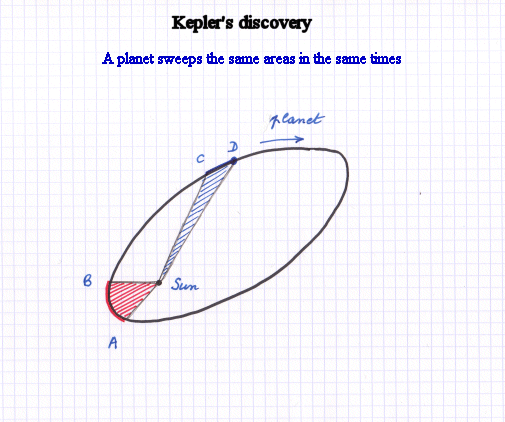
The red shaded surface and the blue shaded surface, if they are sweept in equal times by the planet, have the same area.
Usefulness of the fundamental result of Calculus :
You may wonder so far "OK, these are nice manipulations of mathematical expressions, but why is it useful ?"
Answer : it is useful because quite often it enables us to actually numerically compute an area under a curve.
It applies in a much larger context that just densities of probabiliy. It applies to any "nicely behaved" function (the vast majority of functions used in Finance, Economics, Physics, etc.)
Here is an example of a function f. I chose a simple one. It has a simple explicit mathematical expression : we take x and we square it. It is called a parabola. Suppose we want to compute the blue shaded area under it :
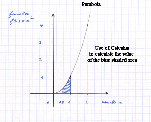
It is easy to verify that the function f(x) = x2 is the rate of variation of the function F(x) = x3/3.
x3/3 is called "a primitive" of x2.
So the surface under f(x) = x2 between 0.5 and 1 is
13 / 3 - (0.5)3 / 3 = 7 / 24
So the blue shaded area ≈ 0.29
Brief recap :
A function F whose derivative is f, is called a primitive of f.
I mentioned casually that a function f cannot have two wildly different primitives F1 and F2. They can only differ by a constant.
We can think of and draw functions for which we don't have a mathematical expression to calculate them. But of course it is nicer to deal with functions for which we have a mathematical expression to calculate them.
There is a special class of such functions that are particularly simple. They are called polynomials. To go from the variable x to the value of the function we only use additions, subtractions, and multiplications. For instance : x -> f(x) = 2x3 -5x +8
Since polynomials are a simple class of functions, it is natural to apply to them the limit process that is so useful all over mathematics.
By a limit process applied to polynomials we mean for instance this : take
the following sequence of polynomials
x
x-x3/6
x-x3/6+x5/120
x-x3/6+x5/120-etc.
(the dividing factor of x2n+1
is the product of the integers from 1 to 2n+1)
Well, the limit of this
sequence of polynomials turns out to be a very interesting function in the mathematics of the
circle, it is called sine of x.
The limit process applied to polynomials yields a large harvest of interesting functions, objects and results. It occupied a good part of the mathematics of the XVIIIth century. And it made mathematicians suspect that there were unifying principles at work to be identified. This lead, in the XIXth century and the XXth century, to a branch of mathematics called Topology, and its rich extensions. Why is it called Topology ? Because to talk about a "limit process" in a space of objects we need to have a notion of distance, so we need to be working in spaces with some sort of topographic structure, "where one can always find one's bearings", and where "to get close to something" has a meaning. The collection of numbers is strongly structured. A collection of socks of various colors is not. The best we can hope for is that we can find pairs :-) The name "topology" was retained for this branch of mathematics.
We also get plenty of interesting functions (useful to represent all sorts of phenomena) when we enrich the permitted operations to division : for instance x -> g(x) = (2x + 3)/(x-1).
Then fractional powers are another natural step. For example :
- x -> square root of (1+x2) , or
- x -> 1 / square root of x*(x-1)*(x-2)
- etc.
Another direction of extension is : functions of things more complicated than one number. And also functions whose values are not simple numbers, etc.
It is customary in high school to explain the simple, though heavy handed, machinery of relationships between one set of values and another set of values, and then... stop when things begin to get interesting. It makes for pupils that don't understand why studying all that has any interest...
It is very easy to compute the derivative of any polynomial function of x. In particular the derivative of powers are simple :
the derivative of f(x) = x2 is 2x. Indeed the slope of the tangent to the parabola, at the point x = 1, is 2. This has a very concrete meaning : if I move a little bit away from 1 on the x axis, by an amount e, the point on the parabola will move vertically by an amount 2e.
More generally speaking the derivative of xn is nx(n-1).
The derivative of xn/n is x(n-1).
By listing all sorts of derivatives we actually are also constructing a list of primitives of course !
The primitive of x2 is x3/3.
The surface area S(x) between 0 and x under a function f is a primitive of f.
So if for some reasons we have at our disposal another primitive F(x), of the function f, from a list, or from any other origin, we know that S(x) and F(x) can only differ by a constant !
So S(b) - S(a) is necessarily equal to F(b) - F(a).
This is exactly what we did with the parabola above :
- We were looking for the area under the parabola between 0.5 and 1
- We happened to know a primitive of the parabola f(x) = x2, because we know the primitives of all polynomials
- It is x3/3
- So we know that the area we are looking for is necessarily 13 / 3 - (0.5)3 / 3 = 7 / 24
This calculation is exact. It's a beauty. The general principle was developped only in the middle ages and after.
Before the advent of computers, to compute an area under a curve f, for which we had an explicit expression, it was necessary to figure out an explicit expression for its primitive F. There are plenty of techniques taught in school to arrive at F. There are also books listing primitives of all sorts of functions. When I was a pupil, finding in a book the primitive to the function we had been asked to integrate was like finding in our Latin dictionary the entire text extract we were toiling upon, translated as an example of use of a word ! For instance the primitive of
f(x) = (1 - x) / (1 + x)
is
F(x) = -x + 2 Log(1 + x)
Now computers can numerically compute F(b) minus F(a) for any function f that "we enter into the computer", without needing an explicit expression for F.
And there also exist formal integrators, for instance http://integrals.wolfram.com/
Example : the primitive of f(x) =
(a+b x+c x^2+d x^3)/(1+x^4)
is F(x) =
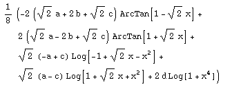
In other words if we draw the curve of F(x), the slope of the tangent to F at any point [x, F(x)] is given by the expression of f(x).
Leibniz introduced his notations in Calculus (they are different from those of Newton), and they are now almost universally employed :
for any function f(x), he noted its derivative
![]()
I don't like this notation because it suggests that the derivative is a ratio and that we can work on the numerator and the denominator like we do with ratios. But the derivative is not exactly a ratio and the suggested manipulations are not always correct.
For the area S under f between a and b, Leibniz also introduced a notation :

It reads "integral of f from a to b".
Here again this notation, beside some advantages, has great defects : it suggest that it is a sum of separate terms and that when applying an operator to S we can compute the result by applying the operator to f and integrate, which is not always the case.
In Mathematics many concepts or "objects" are defined as limits of a series of other objects. For instance : the real numbers, many functions, and areas. Since we are often interested in applying an operator to these limit objects, it is natural to wonder whether we can apply the operator to the elements of the series and apply the limit process (which can itself be viewed as an operator) to the transformed elements by the operator. Sometimes it is OK (most of the time for "well behaved" objects), sometimes not. Some technical chapters of "higher mathematics" are just concerned with studying in which general settings we can do it. They don't really encompass as powerful ideas as the derivation/integration of Newton and Leibniz.
One last word on areas under curves.
Calculus was developped in the XVIIth century independently by Newton and Leibniz. (They spent a large part of their lives disputing who had invented it first.) Then Calculus was greatly extended by other mathematicians in the XVIIIth and XIXth centuries (the Bernoulli family, Euler, Lagrange, Cauchy, Riemann, Lebesgue, etc)
But as early as the middle of the XIVth century Nicolas Oresme had figured out that if we consider the relationship between the speed of an object moving on a line and the time, and we draw a curve representing this relationship (with time on the abscissa axis and speed on the ordinate axis), then the area under the curve between time t1 and time t2 is the distance covered by the object in the time interval.
Oresme was a friend of French king Charles V, who named him bishop of Lisieux, in Normandy, in 1377.
Oresme also made great contributions to the understanding of money. A few years before his birth, the king of France was Philippe le Bel, who is remembered, among other things, for having discreetly reduced the quantity of gold in coins to try to get more money for the State.
Before becoming bishop Oresme headed for several years the Collège de Navarre, founded in 1304, by Philippe le Bel's wife, Jeanne de Navarre. The college was suppressed by the French revolution. Then, in 1805, Napoleon installed the recently created Ecole Polytechnique in the same premises. It staid there until 1976, when it moved to Palaiseau.
A digression within the digression :
Do not mix up great ideas and technical manipulations. Once the mathematician Stan Ulam, surprised by the "lack of interesting results in Economics" asked the economist Paul Samuelson "Can you tell me one non obvious result in Economics ?" Samuelson thought for a time and then came back with the answer : "The theory of comparative advantage of Ricardo". He was indeed quoting a great idea, as opposed to technical manipulations (that in Economics are particularly simple). By the way Ricardo's idea is indeed remarkable, but it belongs to classical economics, a description of economic phenomena that is still too simplistic (too Realist... One could also say too "Mechanistic". Nominalism hasn't yet reached economics, but in fact it took ten centuries to penetrate mathematics, and the work is not completely finished !).
In mathematics, Calculus presented above is a great idea that took four or five centuries to come to fruition. It was then extended in the XIXth century to spaces more convenient than the real numbers, to start with : the complex numbers. Complex numbers extend the usual real numbers so that polynomial equations always have solutions. Eg : x2+1=0 has solutions in complex numbers. Mathematicians introduced complex numbers in the late XVIth century. It took them many centuries to become accustomed to their new creatures, and at first they called them "imaginary numbers". That was still the name often given to them when I was a kid ! Scholars proceeded just like they did with the negative integers, that were little by little introduced in the Middle-Ages (after the introduction of the zero by Indian author Brahmagupta, in 628). Negative integers eventually came to be accepted as natural mathematical objects, and not just "tricks", so that the equation x + m = n have a solution no matter what m and n are (no restriction to n > m anymore). Calculus with complex numbers is a field of surprising unity and beauty, almost entirely developed by one man, Augustin Cauchy (1789-1857).
The introduction of new objects and concepts in Mathematics has most of the time been the fact of users as opposed to pure theorists. This was still the case in the XXth century with "distributions" or with "renormalization" for instance. I remember reputed mathematicians telling me, in 1981, that physicists were doing "impossible things" in some of their calculations. They were talking just like people criticizing Tartaglia four centuries before ! New procedures or objects or concepts were always the subjects of heated debates between their creators and philolosophers, or other mathematicians that did not take part in the creation process :-) For instance the great philosopher Hobbes wrote in several places that Wallis, who participated in the invention of Calculus, was out of his mind !
Calculus, also called Integration, was refined again around the turn of last century (Borel, Lebesgue, Riesz, Frechet, etc.). But it was essentially technical then, to clarify and simplify and extract the gist of some facts. Don't be mistaken : for instance Riesz theorem, stating that linear operators on functions in L2 can always be represented as F(f) = ∫fdm, is the complicated looking statement of a simple geometrical evidence. (One looks first at the effect of F applied to simple functions fa,n worth 1 in the vicinity of a, and zero elsewhere. It gives m. Then any f in L2 is the limit of simpler functions constructed with the fa,n's. And in that space the operators ∫ and "limit" can be inverted. Remember : many mathematical objects are defined as limits of simpler things. That is why Topology came to play such a role in modern maths.)
XXth century mathematics introduced many great ideas, that are of course more remote from common knowledge than those of the previous centuries. For instance mathematicians discovered a deep link between two types of objects they used to study separately, elliptic functions (that extend sine and cosine) and modular forms. This link lead to the solution of a long standing claim by Fermat, by transforming a problem expressed in one setting into a problem expressed in the other setting, for which a solution was found. This is a common way to proceed in mathematics. One could argue it is the way mathematics proceed. Another illustration, among many, that I like, is the beautiful idea of the turn of last century that links the validity of certain long known results in classical Geometry (Pappus, c290-c350, who lived in Alexandria about the time of the Emperor Theodosius the Elder, Desargues, 1591-1661, born in Lyon at the end of the religious wars in France) with the algebraic properties of multiplication in the underlying spaces in which Geometry is considered. Geometry can be studied in fancier spaces than our usual 3D world :-) Probably toys of the future will make this easy to grasp to kids. These ideas of the XXth century sound arcane - that's why I mention them here - but in fact all they require to become familiar with them is practice, just like a cab driver knows his city very well, while a stranger will be at first lost. By the way there is a nice study of the brain of cab drivers published on the BBC website.
Most people afraid of mathematics were just normal kids, that were frightened by their math teachers, that did not themselves have a clear view of their subject.
It took a long time to mathematicians to understand that the concepts and figures they were working with were constructs in their minds first, applied then to perceptions, and not the other way around. In fact they come first from the construct of the integers : one, two, three, etc. There are two apples in this basket ; there are three powers organizing a democracy, etc. Adding the zero, as a "legitimate member" of the same collection, was only done in the VIIth century. All this was finally clearly undestood at the time of Hilbert around the end of the XIXth century.
Of course when we grow up we build in our mind the ideas of lines, planes and stuff like that (mostly because we interact with adults who use the same models). They seem very "natural" because the description of natural perceptions with these constructs works well (only to a point though...). But they don't come from Nature. It is the other way around : Nature is well described with these concepts. I can "demonstrate" geometric problems with the help of pictures on a piece of paper because the piece of paper, as I use it, is a good model for the usual geometry. In fact I really use the pictures as "short hands" for logical statements in english.
One has to be careful though. For instance : if we take a square piece of cloth of side 1 meter and use it to measure the area of a large disk on Earth of radius 1000 km, then we will discover that the area we measured is less than Pi times the square of 1000km. Ok, we will have an explanation, and this will still be explanable within a nice simple "Euclidean space"... But we changed our original view that said : it ought to be Pi times the square of the radius !
The "usual 3-D space" is nothing more than the far consequence of intellectual constructions with integers, multiplication etc. Thales was one of the first to formalize spatial ideas with numbers : he pointed out that figures, when we multiply everything by 2, keep the same shape (an observation that men had made long before Thales, probably more than 40 000 years ago, but they did not care to note it...), and that, with some further precautions, parallels stay parallels, etc.. Fine ! But this is a mental construct, just like saying that there must be two photons to make interferences is a mental construct. By the way this last one had to be abandonned.
There is no need to abandon the usual 3-D space, as well as other "very abstract" spaces or objects we work with to describe Nature (to start with : random variables), but it is important to note that they are all on the same footing : they are constructions in our minds, extending the basic notion of integers.
When we understand all this we begin to take a different view of many problems of humankind : communication, death, individuality, space, what is shown in the Picasso painting below, etc. It's great fun !

This is a vast and beautiful subject that can be approached by the layman in the books of William Feller (1906-1970) "An introduction to probability theory and its applications" Vol I and Vol II.
I will mention only one fact. The density of probability at a value y of a Gaussian with mean m and standard deviation s is given by the formula

There is no closed form expression for the primitive of this function. But there are tables giving Pr{Y≤y} for values of m, s, and y.
And of course, nowadays, there are computers :
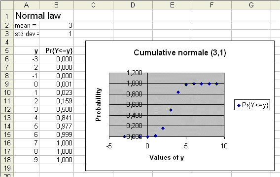
We will not use calculus on densities of probabilities in this course. But we should be aware of the formula above.
We will meet discrete versions of bell curves obtained from establishing histograms.
One point we ought to know about RV and their distributions of probabilities is this :
- the simplest RV are discrete finite RV
- continuous RV are less easy to manipulate (for simple analyses)
- it is possible to study any kind of continuous RV, coming from real life applications, by transforming them first into discrete finite RV
- but it turns out that when we want to carry out elaborate analyses on continuous RV it is easier to deal directly with their densities of probabilities than to transform them into discrete ones first and then work on their discrete distribution of probability.
That is precisely for the same kind of reasons that Calculus is so universally used in Physics, Economics, Finance and many other fields.
It is one illustration of the ambivalent relationship between "discreteness" and "continuity" :
- at one level the first concept is simpler : counting is simple
- but at another level the second concept is simpler : smooth functions and their closed form expression are often simpler than finite collections of numbers to deal with !
For instance it is easier to deal with the function x-> f(x)=1/x and its integral ∫1 to x f(y)dy = log(x), which with some practice is simple, than with the sequence 1, 1/2, 1/3, 1/4, etc. and its sum S i=1 to n 1/i which remains messier.