Wednesday November 10th 2004
Finance : fifth lecture (part one).
Introduction
The Internal Rate of Return is an extension of the concept of profitability of a
security
Opportunity cost
of capital of an investment I
Risk pattern and risk of an investment
The set of future cash flows of an investment should be viewed as a whole
Continuous model
Net Present Value of I
NPV and IRR
Selling an investment
The material we study in this Corporate Finance course is relatively recent. It was developped in the 1950's, 1960's and early 1970's.
Of course Finance is older than that : the idea of gathering large amounts of capital from several private partners to set up a risky venture (one of the central ideas of capitalism) goes back at least to the large Trading companies of the early XVIIth century (for instance The Dutch East India Company, Amsterdam 1602) ; and the limited liability acts, that helped the spur of capitalism, were passed in all western countries in the mid XIXth century. Even before that, the first stock markets, where securities of various sorts (we saw that they are always debts of someone) were traded, were created in the XVIth century (for instance Paris, 1563). And some early places of exchange appeared even before that period.
But the clear understanding and description of what we mean by the risk of a security was achieved only in the 1950's (Harry Markowitz, 1952). The current standard theory of portfolio management (that is how to best spend our money into a basket of securities in the stock market) dates from the sixties (Capital Asset Pricing Model). The calculation of the correct pricing of options dates from the seventies (Black and Scholes, 1973).
Secondly, the world of Finance underwent tremendous changes in the last 30 years. At the beginning of the XXIst century, pension funds and other kinds of syndicated investment tools account for more than 50% of the entire stock ownership, as opposed to about 15% in 1950. New sophisticated investment vehicles, derivatives, swaps, options on indices, etc. appeared in the last twenty years. Hedge funds thrived in the 1990's. The single individual stock market player reading carefully his financial magazine, paying attention to the journalist recommandations... , and deciding how to modify his stock and bond portfolio (like my grand uncle Albert Fabry did) is a Norman Rockwell image of the past. Individual investors account today for only a few percent of the market.
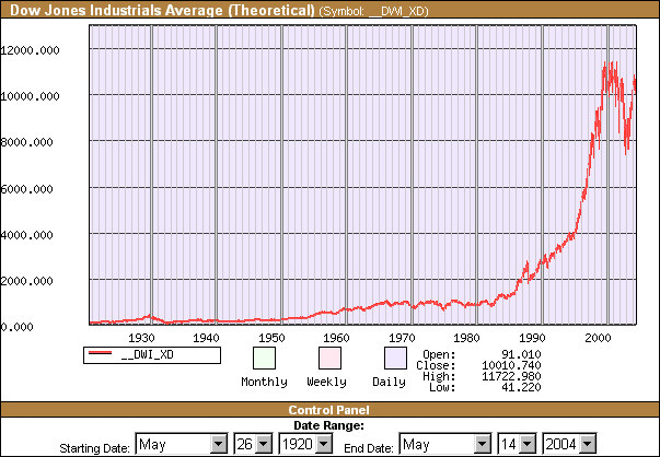
And, as we know, the world financial markets of today are rather unstable. When we view the graph of the Dow Jones index below, we must admit that
Source : http://www.globalfindata.com/
All this suggests that Finance ought to be terribly difficult.
What is true is that, at present, no satisfactory theory explains what governments should do to stabilize the stock markets, or even whether this should be considered a problem. Yet most observers admit that it is a problem, that it is linked to big financial crises like the Asian crisis of 1997/98, that it hampers world prosperity and fair sharing of wealth (we know that we are far from these objectives !) and that new world financial structures and tools (a new money perhaps ?) are probably called for.
Because of the difficulties run into to explain and drive economics, some people call it "the dismal science" and foretell that it will never improve. We do not share this view. After all medicine too deserved the name of dismal science until the XIXth century. The progress brought by Galien, Ibn Sina, Paré or Harvey were scant. Molière used to make fun of the physicians of his time (Diafoirus). The major remedy they knew was to bleed people. The only positive comment that can be made about this remedy is that... it selected the sturdiest. Mind you, economics did not do much differently to try and get out of the great depression of the 1930's, until Keynes suggested a new type of government intervention, the real efficacy of which is still, to this day, hotly debated.
Yet Jenner discovered vaccination in 1796. Pasteur launched immunology in the late XIXth century. Fleming discovered antibiotics in the 1928. Medicine was revolutionized by these men and a few other people. Many new ideas, that required a Nominalist understanding, as opposed to a Realist understanding, of the world, were successfully introduced. One striking consequence is that average life expectancy was multiplied by two over the XXth century. Now medicine is no longer a dismal science. Yet it can be argued that medicine addressed problems more difficult than those facing economics. So there is hope.
New, more efficient, theories of Economics, Money, and Economic policy will be developed using the tools elaborated in the theory of Complex Dynamic Systems. This will be one of the grand scientific achievements of the XXIst century. It requires investigating and understanding systems that display intrinsic instability, with strange attractors, and upon which actions guided by intuition derived from linear toys are countereffective.
Anyway elementary Finance is not difficult. The basic tool to evaluate investment projects, Discounted Cash Flow analysis, is a simple way to take into account the riskiness of expected future cash flows, and is fairly easy to master at a practical level. It is today's topic.
Most of the definitions and calculations we shall deal with are extensions of those we made on securities, to investments producing a sequence of cash flows in the future.
The Internal Rate of Return is an extension of the concept of profitability
In the preceding lectures we studied at great length the behavior of a security S from one year to the next. S has a price P today, it will have a value X in one year. X is a random variable with an expectation
E(X)
and a variability measured by its standard deviation :
sd(X) = square root of E{ [ X - E(X) ]2 }
The profitability of S is the random variable
R = ( X - P ) / P
R has a mean E(R), that we denote rS.
and a standard deviation sd(R), that we denote σS
Language abuse : often when we talk about the profitability of S, instead of R, we mean rS.
rS, the profitability of S, has a nice simple property : it is the value of the variable r, such that
[E(X)/(1+r)] - P = 0
E(X)/(1+r) is called the Present Value of E(X) calculated with the discounting rate r.
And [E(X)/(1+r)] - P in called the Net Present Value (NPV) of investing into S calculated with the discount rate r.
So we see that NPV of investing into S is a function of r. We can denote it
NPV(investment into S ; r). For each value of r, there is a value of NPV(investment into S ; r)
Example : P = 50€, E(X) = 65€, then NPV(S ; r) is the following function :
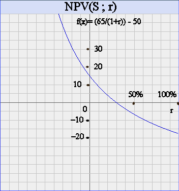
Here NPV(S ; r) is zero for r = 30%.
More generally, rS is the value of r such that the NPV of investing into S is zero.
Recap : for an investment of a sum of money P into a security S that will yield in one year a random value X, and a profitability rS, it turns out that this last figure is the variable r such that the NPV(investing into S ; r) is zero.
This fact allows us to generalize the concept of profitability of an investment, to investments that will yield a series of cash flows.
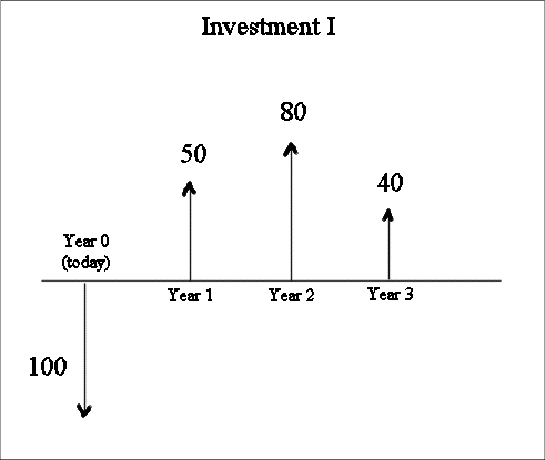
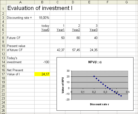
Here is an example : let's consider an investment I. The sum of money to invest at the beginning, at "year 0", is 100 million euros. It is called C0. And this investment will produce three random cash flows which have expectations C1, C2 and C3 : 50 million €, 80 million € and 40 million €.
Here is a representation of I :
Now the concept of profitability of I is no longer as simple and natural as in the case of an investment with a single value one year later.
We cannot either just add up 50+80+40 (=170) and say the profitability of the investment is 70% !
Here comes in the nice property of the profitability of a one-year-investment, because it lends itself to a natural extension. This time we won't go into all the probabilistic justifications of the following treatments. But their character will be natural and intuitive.
Consider a variable discounting rate r.
We shall call "the Present Value today of C1, discounted with the rate r", the quantity C1/(1+r).
We shall call "the Present Value today of C2, discounted with the rate r", the quantity C2/(1+r)2.
We shall call "the Present Value today of C3, discounted with the rate r", the quantity C3/(1+r)3.
And NPV(I ; r) is defined as the sum of the three present values minus the initial investment:
NPV(I ; r) = C1/(1+r) + C2/(1+r)2 + C3/(1+r)3 - C0
It is a function of r.
Here is its graph :
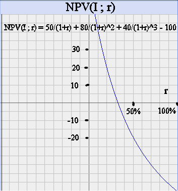
The curve of NPV cuts the horizontal axis, that is is equal to zero, when r is somewhere between 30% and 35%.
The exact value is r=32.87%. It can be obtained using the goal seek tool in Excel. Or it can be obtained more or less precisely by trial and errors with values of r between 30% and 40%. It can also be estimated rather precisely by graphical techniques : compute NPV for r = 30%, we get 4.01 million euros. And compute NPV for r = 40%, we get -8.89 million euros. A linear interpolation in between yields the root r = 33.1%. It is not the exactly correct number (which is 32.87%) but it is not bad.
This value r = 32.9%, which makes NPV(I ; r) = 0, is called the Internal Rate of Return of I.
It is a generalization of the concept of profitability of an investment to a situation where the future value is not unique, but is a series of several yearly cash flows.
Recap : by definition, the Internal Rate of Return of an investment I with initial cash flow in C0, and subsequent cash flows out C1, C2, ... Cn, is the value of the discounting rate r, such that NPV(I ; discounted with r) = 0
(Note if we have the following set of cash flows : [ -P , P*ρ , P*ρ , P*(1+ρ) ] it is easy to check that the IRR is r = ρ. So this confirms that the IRR is a natural extension of the concept of profitability.)
Opportunity cost of capital of an investment I :
The previous section explained what is the IRR of an investment. It is a figure that is calculated purely internally from the sequence of expected cash flows, C0, C1, C2, ... Cn.
Now comes another important discounting rate related to the investment I.
Recall that in the previous lessons we explained what we mean by "two securities have the same risk pattern".
The notion of "same risk pattern" can be extended to investments producing more than one unique cash flow one year later. The mathematics are more intricate than for a security producing a unique cash flow in one year, but the intuitive idea remains simple : equivalent risk behavior.
Digression : Risk pattern and risk of an investment :
For a security S we were able to define its risk pattern without any reference to a price : it was E(X)/sd(X), where X is the random value of S in one year.
And we defined the risk of S as the standard deviation of its profitability.
For an investment with an initial cash flow C0 invested and three (or more) expected cash flows C1, C2, C3 produced in the future, it is no longer straightforward to define a risk pattern without reference to its price (here C0). Yet it is possible. And it has to be, otherwise how would we decide what to pay for a set of future cash flows ?
(We strongly disagree for instance with Brealey and Myers, who write on page 98 of edition 6 of their textbook, that "interpretation [of opportunity cost of capital] is not always easy for long-lived investments projects".
The risk pattern, as well as the opportunity cost of capital, of an investment must just be defined, no "difficulty" about it. There are several ways, the simplest one is to consider the IRR as a random variable and then treat things like for one security. One has first to be clear about the probabilistic model for the investment.
It reminds us of the Accounting author, John Dyson, who writes, in the same vein, that "computing the unit cost of a product in a multi-product plant is difficult". It is not "difficult", it just has to be defined, and, like any definition, it is done with some purpose in view.
We also met in another well-known Accounting book, by Weygandt, Kieso and Kimmel, page 45 of edition 6, this surprising sentence "the term debit means left, and credit means right", ignoring entirely the natural appearance and explanation of these concepts when, around the XIIth century, merchants began to feel the need to record in a systematic and convenient way sums owned and owed but not yet paid, and invented double-entry accounting - such a fine method that to this day it is still used without essential change.
One should know what knowledge means ! Everything we talk about must be clearly defined, otherwise we are confused, and confusing. And when concepts have a clear historical origin, explaining this origin is usually quite useful.
Kolmogorov clarified probability forever when he said : "The theory of probability ... can and should be developed from axioms ...", and did it in the 30's of XXth century.)
On the other hand defining the risk of a multi-cash flow investment is a natural extension of what was done for a security :
For each actual outcome of the three future cash flows - let's call them X1i, X2i, X3i - there is a value Ri such that the Present Value of the three cash flows is equal to C0. It is an outcome of a random variable R.
This random variable R has an expectation E(R), that turns out, if we stick to a reasonable probabilistic model for the future cash flows of our investment, to be the IRR of I (that is : we can reverse the order of the "IRR operator" and the "Expectation operator" on the random variables), and it has a standard deviation. This standard deviation of R can be the definition of the risk of I.
Then we have the tools at hand to compare I and S. But only if we already have a price for I (namely C0).
This gives a glimpse of the theoretical difficulties encountered with the risk of I and its comparison with the risk of S, but we shall not concern ourselves with those here.
The set of future cash flows of an investment should be viewed as a whole
An investment is a financial action (investing a sum C0 into various assets acquisition and putting them to work) that will produce an effect : generation of a collection of n yearly cash flows.
These future cash flows should be thought of "as a whole", and not only as a sequence of individual payoffs, one after the other.
The traditional way of viewing them as a chronological sequence of individual payoffs, even though it is technically correct, makes the analysis of the investment more difficult to comprehend.
A comparison will make this clearer : not seeing the future cash flows as a whole but as a series of individual payoffs is like staunchly thinking of unit costs in a factory making different types of products. We can define unit costs but they are somewhat artificial. At first what is factual is that we have a factory driven by a set of costs and producing a set of series of products. The costs are not simply related to the products. Only the set of different series of products is related to the set of costs.
Then, for various reasons (including deciding unit prices, that can be, by the way, an elaborate price list) we define/calculate somewhat artificially unit costs, but it is easier to understand the cost model of the factory if we think of the costs as a whole linked to the set of series of products as a whole. On the contrary if we stick to a mental view of unit costs per product we run into all sorts of difficulties to figure out how they change with a new production schedule. And that is because the cost model is not naturally structured with costs per product but with costs per department.
Same is true of the set of future cash flows produced by an investment.
(One of the usual models for the n future yearly cash flows generated by investing C0 today, is : they are n independent random variables with increasing risk pattern. Why not ? But when one thinks of it, it is not a particularly realistic model. Anyway we shall not concern ourselves with the details of the model used to analyze our investment.)
By definition, the opportunity cost of capital of an investment I is the profitability of a security S traded in the stock market, and that has the same risk behavior as I.
Customarily, we take for S a security in the same industry as I, or the average profitabilities of securities in the same industry as I.
When we were offered a security T which had an expected future value E(Y), but no price PT today yet, and which had the same risk behavior as S, for which we knew the profitability rS, we computed the price of T as
PT = E(Y) / (1+rS)
that is we discounted the expected future value of T by its opportunity cost of capital to compute the maximum price we should be willing to offer for T today.
This extends to the investment I with initial cash flow in C0, and future cash flows out C1, C2, ... , Cn. We find in the stock market a security S which has the same risk behavior as the set of future cash flows of I. The profitability of S is called "the opportunity cost of capital of I", because if we don't invest into I we can invest into S and incur the same risk, and have a profitability rS. So it's an equivalent "opportunity" that give up.
DCF analysis tries to represent the way investors choose between two investments possibilities.
In the case of a choice between two securities that will each produce one random cash flow in one year, the modelling is rather simple : we use the rule stating that between two securities with the same expected future value in one year, investors will pay more for the one that has less variability. The DCF calculations are a straightforward consequence.
In the case of a choice between two securities that will produce their future random value at different times, for instance the first one in one year and the second one in two years, the situation is a bit more complex. We have to model the way investors "approach time", whereas in the case above it is not necessary : we just compared two securities at the same time, so the effect of time did not matter much to us.
The standard answer is this : if investors are willing to equate P today with a random cash flow X1 in one year, where X can be written
X1 = P*(1 + R1)
then they should also be willing to equate this X1 in one year to X2 in two years, where X2 = X1*(1+R2), where R2 is a random variable with the same behavior as R1. (This is the extension of the rule stating how investors choose between two securities, to securities that don't produce their cash flows at the same dates.)
That is why X2 in two years is considered equivalent to P today. And since E(X2) is equal to P*(1+r)*(1+r), where r is the expected value of R1 and R2, we discount X2 the usual way to get P :
P = E(X2) / (1+r)2
This is the common presentation and justification for DCF.
Note that X2 has a higher expectation than X1 and has also more variability than X1. So investors consider equivalent P today, or X1 in one year, or X2 in two years.
The model raises plenty of questions and paradoxes : for instance "should we use the same r ?"
The only way to clarify satisfactorily all this is to develop a continuous model for the future value of the security over time, with the use of Calculus.
Remember that, stated very loosely, Calculus is a mathematical technique to deal with quantities that are the result of a multiplicative process where the multiplicands vary all the time. (See lesson 2b for details.) This is the case of the future value of a security.
We will have (Value of S at time t + dt) = (Value of S at time t) *( 1 + R(t, dt)), where R(t, dt) is a random variable the distribution of which depends upon time t, and interval dt.
When dt tends to zero, if S is a government bond, R(t, dt) tends to the risk-free rate at time t ; otherwise R(t, dt) tends to some value higher than the risk free rate.
This requires simple stochastic calculus, and we shall not treat it here.
One more point to remember : the passage from discrete to continuous models requires to master elementary calculus, it is a preliminary barrier, but then everything is much simpler in continuous models than in discrete models.
We shall now discount the future cash flows of I with its opportunity cost of capital. The result will be called "the Present Value of the future cash flows of I" (with no more reference to a variable discount rate), and when we subtract C0, we call the result "the Net Present Value of I".
Before, we considered any variable r, and discounted the future CF's with r, and we obtained a quantity NPV(I ; r) function of the variable r.
Now we consider a fixed meaningful r, which is rS = the opportunity cost of capital of I, and we define a unique NPV(I) = NPV(I ; rS)
Recall : the formula is
NPV(I) = -C0 + C1/(1+rS) + C2/(1+rS)2 + ... Cn/(1+rS)n
It reads "the Net Present Value of I is ..."
This is not complicated, but we have to pay attention : just like in the case of one security T,
C1/(1+rS) + C2/(1+rS)2 + ... Cn/(1+rS)n is the maximum price someone should be willing to pay for this sequence of future cash flows.
If for some reason we can generate them by investing a sum C0 today that is less than the above figure, we are in a favorable position : we can make an investment with a positive NPV.
Moreover, let's think of our situation just after having made the investment I, that is just after having spent C0 : according to this standard financial model, we should be able to find someone willing to buy from us all the concrete realizations of this investment for the sum C1/(1+rS) + C2/(1+rS)2 + ... Cn/(1+rS)n . Therefore we are in a position, so standard Finance says, to earn right away the NPV of I.
Stated another way : if we can make today an investment I with a positive NPV, we are potentially richer by this amount today. That's an important point : it is not after the investment is finished (in three or more years) that we are richer; it is right now. We can find someone willing to buy it from us for the sum of the discounted expected future cash flows ; we make it for C0 ; and we keep for us the difference, namely : the NPV.
The NPV of an investment I is positive if and only if its IRR is higher than its opportunity cost of capital.
Indeed, remember that the IRR is that value of the discount rate r such that NPV(I ; r) is zero. Since, except in odd situations (that some textbooks like to insist upon, probably because they did not understand the deep logic of all this, and they try to compensate by producing false complexity) with no Financial relevance, the function NPV(I ; r) is decreasing with r, we see that if we discount with an opportunity cost of capital that is less than the IRR we get a positive figure.
In other words, the standard theory of Finance says : an investment I is a good investment when its Internal Rate of Return is higher than its opportunity cost of capital. In that case we should go ahead and make the investment, unless we have a better one yet.
Take the numerical example considered above. Suppose it is a "plain vanilla" investment in the commodity chemical industry, and that the average profitability in this industrial sector is 18%. Then this is the opportunity cost of capital of the investment I. It is lower than 32.9% so we know that it is a good investment, with a positive NPV. Its NPV is given on the graph
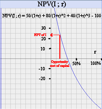
It is about 24 million euros.
If we make the investment I, we can earn this money right away by selling the investment (once made) to someone else, that should be willing to pay to us 124 million euros.
Why someone else should be willing to pay us 124 million euros to acquire the facilities created by the investment ? Because for that person the investment will produce
C1 = 50 million €, C2 = 80 million € and C3 = 40 million €
(Remember, in the standard Financial framework, these figures are expected future cash flows. There is a simple probabilistic model for the behavior of the investment I in the future. Some firms financial departments like to study the projected investment and its various financial characteristics using Monte-Carlo simultations. This is a big word to say "simulations on a spreadsheet using a random number generator". It is indeed very convenient to get a feel of how the investment may unfold. It is an extension of what we did with Excel to study the profitability of a security.)
And this is an investment in the chemical industry, therefore it has a risk behavior like stocks in the chemical industry, their profitability (for the sake of this lesson... ) is 18%, so that is its opportunity cost of capital for our buyer. He makes the computation, that is he discounts these expected future cash flows with 18% and gets 124 million euros. So he is willing to pay that to us for it.
Here is are the calculations made by us and by our potential buyer (except that he is not supposed to know our C0 ! All he knows is that the three future CF have a value today of 124 million euros.)
We just saw that for a potential buyer our investment, once we have made it, should have a value of 124 million euros. In fact this is a minimum value : indeed if for some reason acquiring this investment will allow our potential buyer to reduce some other costs in his industrial activities, he should be willing to pay even more than this for the investment, because his view of the cash flows will be different from ours. He'll see savings we won't see. On the other hand he does not know that for us the initial investment is only C0 = 100 million euros.
This is an illustration, in a financial setting, of the economic and accounting fact that the same assets don't have the same value for everyone (see lesson 1 section "Value is not the same for everyone".)
Of course, there remains the question of "where does our possibility to have a positive NPV come from ?". This is a question in Economics more than in Finance. It is correctly answered by a model of a community of actors producing, exchanging and consuming, each having personal prices. It is outside the scope of this elementary course in Finance.
Break time