Wednesday November 10th 2004
Finance : fifth lecture (part two).
A note on spreadsheets
New ideas
Computing the IRR of an
investment
Let's figure out the IRR using a geometric linear interpolation
Let's use Excel "goal seek" tool
The risk pattern of J
The opportunity cost of capital of J
Is J a good investment ?
The importance and the relativity of the future cash flow figures
Case when a buyer is willing to offer more than the Present value of the future
cash flows
What is to be included in the computation of the future cash flows of an
investment requires some care
Buying an investment to kill it
Bonds
Why bonds yield more than the risk free short term rate ?
Risk pattern and opportunity cost of a bond
Present value of the stream of coupons plus the final refund
What happens when the interest rate offered by the market changes ?
We have been using extensively the spreadsheet Excel to make computations on the investment I.
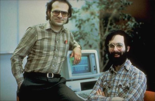
Spreadsheets have an interesting story. The first spreadsheet was created by two students at Harvard, Dan Bricklin and Bob Frankston, in 1978. They were in the MBA program and had a lot of repetitive calculations to make, like studying a budget under varying hypotheses or studying the profitability of an investment depending upon its opportunity cost of capital.
Here are Frankston (left) and Bricklin (right)
At the time they were using hand held calculators, and they thought (it's Bricklin that is credited with the initial idea) of having some sort of virtual calculator simulated by a software on their home Apple II computer : it would have a grid of cells that would be represented visually on the screen of the computer. It would be possible to enter numbers or formulas in the cells, and changing one number parameter and updating the whole calculation would be very easy...
Here is the Apple II :
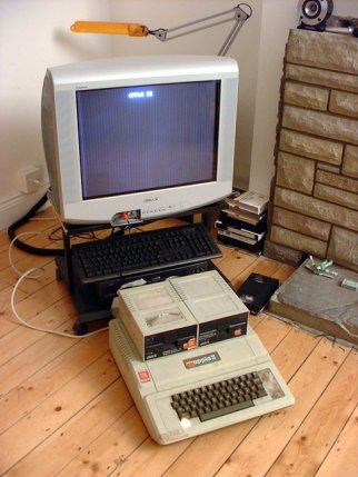
And here is one of the first versions of Visicalc, the name of the software Bricklin and Frankston developed on the Apple II.
In the late seventies home micro-computers like the Apple II were still considered mostly to be super kids toys, or funny tools for scientists beside the main frames they had access to in their research centers. They had not penetrated the offices of the business world.
But after Visicalc and some other "killer applications", like the word processor, business people began to use these "toys", and little by little began to realize what fantastic enhancement they provided to the work of their office assistants and to their own work.
In 1979, while a math teacher at MIT, I remember that the secretaries used plain old typewriters to type our research papers. And in 1981, when I became a consultant at the Boston Consulting Group, the secretaries were using "advanced typewriters" equipped with some storage device using large floppy diskettes to store their work and modify it easily. Soon after that, they changed for personal computers that the firm bought for them. And the consultants began to use them as well...
The tremendous success of Visicalc is one the causes of IBM decision to enter the micro-computer business, after years of snubbing it. The story of the IBM PC project is as exciting as the best thrillers.
And the launch of the IBM PC spurred the growth of micro-computers, which in turn was a necessary prerequisite for the worldwide development of Internet, which is changing our lives...
It is always a fruitful effort to try to figure out what a tremendous insight it required to invent such a tool, so familiar to us today, as a spreadsheet on a computer screen.
The same is true of Oresme's idea of "representing concretely" the abstract relationship between two quantities f and x as this : for each x, let's position our pencil on a horizontal axis at a distance x from an origin, and let's raise a vertical distance f(x) and draw a dot on the point we reach. With all the dots, we obtain a curve (blue, on the picture below) :
Today this representation seems so natural to us that we forget how daring it was to devise it. Oresme said "it gives some sort of concrete representation of the abstract relationship between the quantities we want to study, and it turns out to be very useful".
At first it was indeed very remote from what people thought of what a relationship is. For them "a relationship" was something very abstract, and the idea of having a concrete representation for it was even... more abstract.
Then Descartes developed Oresme's idea. He realized that the "Oresme representation" of functions having a simple algebraic expression (like f(x) = 3x2 - 5x + 7) transformed nice algebraic properties into nice geometric properties, and conversely. But for this development to take place, the ideas of algebra had to become familiar in the West too. One of the first book on algebra is Al-Bahir fi'l-jabr, published, in 1149, by Ibn Yahya Al-Samawal.
A lot of mathematics, and a lot of "understanding" for that matter, simply consist in taking one setting of structures and transforming into another setting of structures with which we are more familiar and comfortable. And, naturally enough, what we figure out in the transformed setting corresponds to unsuspected facts in the first setting.
New ideas are always disturbing at first. They appear farfetched, remote, difficult, unbelievably cerebral. And eventually it becomes something everybody is used to. It is true for "representing" sounds and words and speech, like I do and like you are reading right now. And it is true for "non commutative algebras" like Alain Connes invented in the 70's to represent some physical processes where we cannot reverse freely the order of the operators : abstract, isn't it ? Only until we become used to it ! And how to get used to it ? Answer : by hours of practice.
One last point I would like you to remember : new ideas are often surprising at first, but they are always simple. If you read about new ideas and they appear confusing, either the author goes too fast, introduces too many new ideas at the same time, or he does not really understand them. In either case go to a better book, and things will become clear.
There is no such thing as a complicated idea. But most new and powerful ideas require to put a lot of time to become familiar with them. Don't expect to master new tools without work :-)
Computing the IRR of an investment :
Consider the following investment J
C0 (the money to invest at the beginning) = 120 million €
Then we get four random cash flows with the following expected values :
year 1 :
C1 = 30 million €
year 2 :
C2 = 50 million €
year 3 :
C3 = 50 million €
(Erratum : In a previous version of this lesson
there was a fourth year with a cash flow C4 = 10 million €, but then it got omitted in the subsequent
DCF calculations, leading to erroneous results.)
What it the IRR of J ?
(Remember : the IRR of J is the extension to a series of cash flows of the familiar notion of profit of a security producing one cash flow next year.)
Before diving head on into the computations, let's stop for a moment : We may note that this investment does not produce a lot of money ! 130 million € over three years, and we have to invest 120 million € at first to produce this. Its profitability cannot be very high. So it better be not too risky.
Note too that we are not given any information yet on the riskiness of this investment. How risky is it ? We don't know. For that we will need extra information. If it is too risky, we know that J won't pass the test "Is it a good investment ?"
But right now we are not concerned with that (and - I repeat - anyway we don't have all the information necessary to check whether this is a good investment or not).
All we want to know is the IRR of J. This is an "endogenous" figure. It does not require any extra external information to be computed. It is just an extension of the concept of profitability of a security. Like if you invest $50 and get one year later $70 on average, you know that you have a profitability of 40%. No need for extra information about the risk of that security.
To get at the IRR of J, let's try a first discounting rate r = 10% :

We get a NPV of -13.84 million €. So the IRR of J is less than 10%.
Let's try 5% :
Still too high !
Let's try r = 2%.
By the way if J does not "pass 2%", it will be rejected for sure, because 2% is the rate required from risk free investments, that is those the cash flows of which are sure (with no variability whatsoever).
Ok, the NPV computed with r = 2% is positive. So the IRR of J is higher than 2%.
Let's figure out the IRR using a geometrical linear interpolation :
From our high school geometry we see that
x/4.59 = (3 - x)/2.89
this gives
x times 2.89 = (3 - x) times 4.59
x times (2.89 + 4.59) = 3 times 4.59
this gives x = 1.84
Our estimate of the IRR is then 2% + 1.84% = 3.84%
Here is a graph of the NPV as a function of r :
"Linear interpolation" is nothing more than treating a curve, locally, as a straight line, and applying simple facts from the geometry of triangles (developed by Thales, circa 624 bc - circa 547 bc).
Every nice curve "if you look closely" looks straight :-)
Finally, to get a precise estimate of the IRR, let's use the "goal seek" tool of Excel :
At the time of Bricklin and Frankston spreadsheet did not have this nice functionality. But there has been a lot of developments on spreadsheets. Now they are more or less a mature product that does not evolve very much any more. However, spreadsheets are often the hidden basis of other applications, either applications targeted to specific industries, or applications achieving more specific goals than plain spreadsheets (for instance, simple accounting softwares that you can find on store shelves). A whole industry of application developers sprang up. The same is true of databases : there are the standard products, and there are plenty of commercial products that use a (hidden) database behind the scene (Access or other databases).
Here is the goal seek tool at work :
The precise result is : IRR of J = 3.81%
Note that this is done "for the beauty of the work well done". In Finance we rarely care for such precise estimates. 3.8% (and even, sometimes, "about 4%") is good enough.
So far we were not told what is the risk pattern of J.
By "what is the risk pattern of J" we mean "what security, that we know, has the same risk pattern as J ?".
In practice, we need to know more about J to answer this question :
- usually : "in which industry does it take place ?"
- or, alternatively, "do we have a complete probabilistic model for the behavior
of the future cash flows ?" In this case we can compute the probabilistic
behavior of its IRR computed from actual outcomes of the cash flows. But it is a rare situation
in financial practice, and we won't study it in this
course.
Opportunity cost of capital of J :
Suppose we know that J has the same risk pattern as the securities in the electric utility industry. And we know (for the sake of this lesson) that those securities all have profitabilities around 6%.
Then this figure of 6% is the opportunity cost of capital of the investment J.
No. J is not a good investment.
Why ? Because its opportunity cost of capital is higher than its IRR, so we know that the actual NPV of J is negative.
This means that "The value today of making this investment is negative". Said another way : "Putting 120 million euros in investing into J, in order to get the three cash flows above, with the risk of the electric utility industry, is a waste of money."
Exercise : compute the NPV of J
(Answer : -5.22 million euros)
The importance and the relativity of the future cash flow figures
It is important to note that, even given the opportunity cost of capital of J, the calculations above depend heavily upon the future cash flow figures as well as the initial cash flow.
For instance if C2 and C3 are revised to 60 and 60, instead of 50 and 50, then all the calculations and the conclusions change (even without changing the opportunity cost of capital) :
Now the NPV of J, calculated by discounting the future cash flows with its cost of capital of 6%, becomes +12.08 million euros.
In that case J becomes a good investment for us.
We could make it and keep it for us. Or we could sell it to somebody else for 132.08 million euros.
Case when a buyer is willing to offer more than the Present value of the future cash flows :
Suppose that after having revised the precise forecast budget of our investment we find that its NPV for us is 132.08 million euros.
There may be cases where a buyer is willing to pay even more to us that 132.08 million euros.
It is not because he makes a mistake in his DCF analysis. He makes it as correctly as we do. But he may have different cash flows !
Why does he have different cash flows ? Because, perhaps, by acquiring the project from us, he will no longer need certain expenditures that are already taken care of with the investment.
What is to be included in the computation of the future cash flows of an investment requires some care : for instance if the investment includes new premises we will move into, we should include in the cash flows the rent we will no longer pay elsewhere. Similarly if the potential buyer sees other savings for him, he will include them in the cash flows.
Suppose that a potential buyer sees for him the following expected future cash flows :
30, 65, 65
In that case, for him the project has a positive NPV as long as he purchases it from us for less than 140.73 million euros.
So he may very well offer us a price of 137 million euros. We agree. We sell the project to him for that price. And every body is making a good deal !
Buying an investment to kill it :
This may come as a surprise, and may (correctly) shock our sense of ethics, but in the world of business there are plenty of examples where a large firm purchased a smaller one, or purchased a project, with the clear intention of not developing it !
Why ? Because, the small firm would, or the project would reduce to insignificant numbers the future cash flows of another big project the firm has already invested in.
And the NPV of buying the new firm (even at a significant price) and not develop it is highly positive !
Exercise : Come up with examples.
We finish up this lesson with a first overview of bonds.
What is a bond ?
It is a financial contract between a borrower (usually a firm) and a lender (an investor) according to which :
x% is called the interest paid by the bond.
the yearly payment of x% times $1000 is called the coupon.
n, the number of years, is called "the maturity" of the bond.
Bonds are simple financial contracts. They are simpler than stocks.
Why bonds yield more than the risk free short term rate ?
For two reasons :
So we want more than the short term risk free rate.
In fact if we were to accept the risk free rate, "because we are absolutely sure of the borrower, and also of the money", nothing forces us to sign right away a say seven year contract with the borrower. We can always reconduct a yearly contract. We lose nothing, and we gain the possibility of changing our mind.
Risk pattern and opportunity cost of a bond :
We won't go into all the probabilistic justifications for it, but the risk pattern of a bond is that of a security the yearly profitability of which is the interest rate of the bond.
In other words, the opportunity cost of a bond is its interest rate, as long as it is the interest rate offered by the market for similar bonds did not change.
Here is the schedule of payments of a 6% 8 year maturity bond :
| Bond | ||||||||||
| Interest rate = | 6,00% | |||||||||
| Today | Year1 | Year2 | Year3 | Year4 | Year5 | Year6 | Year7 | Year8 | ||
| Future CF | 60 | 60 | 60 | 60 | 60 | 60 | 60 | 1060 | ||
| Today's investment | -1000 | |||||||||
Present value of the stream of coupons plus the final refund :
The opportunity cost of a new bond is its interest rate. (The alternatives with the same risk pattern have this profitability.)
So the Present value of the stream of coupons plus the final payment is
60/(1+r) + 60/(1+r)2 + ... + 60/(1+r)7 + 1060/(1+r)8
with r = 6% it is precisely equal to $1000.
You are invited to check the numbers by yourselves :
| Today | Year1 | Year2 | Year3 | Year4 | Year5 | Year6 | Year7 | Year8 | |
| Present values | 56,60 | 53,40 | 50,38 | 47,53 | 44,84 | 42,30 | 39,90 | 665,06 |
Sum of these values = $1000.
And it is a simple algebraic exercise to show that this is always true.
What happens when the interest rate offered by the market changes ?
That is when things become interesting :
you hold a bond bought sometime ago (say 2 years ago, and it was then an 8 year bond). And suppose the interest rate that you get by contract is 6%. As far as the time aspect of the contract is concerned your old bond is like a new bond with a shorter maturity (6 years).
But if new 6 year maturity bonds are issued now with an interest rate, set by contract, higher than 6% (because the market conditions changed), say it is now 7%, your old bond is not exactly equivalent to a new 6 year maturity bond.
We shall see in a subsequent lesson, after the mid term examination, how much is your old bond worth now.