Wednesday November 17th 2004
Finance : sixth lecture.
Introduction
A RV simulating the payoff of a security
case 1 : we know the underlying distribution
case 2 : we don't know the underlying distribution
Digression on Statistics
The Polyzone project
Monte-Carlo methods
Profitability and IRR
Risk and opportunity cost of
capital
Digression 1 : Ronald Coase
Digression 2 : The objectives of Economics
Erratum
Today's lecture is a review, in preparation for next week mid term examination.
We will review working with a discrete random variable simulating the payoff of a security. There will be two cases : the case where we know the "underlying probability distribution" and the case, closer to situations in real life, where we don't know the underlying distribution.
Then I'll present a nice application of DCF analysis to the evaluation of a large projected investment in the chemical industry ; how we use it to forecast the likely behavior of competitors ; and how it leads to a revision of the initially planned prices. This fine example is taken from the textbook by Brealey and Myers.
We will present Monte-Carlo methods in a simple example : calculate the area of a quadrant of disk, inscribed in a square, by "throwing" 50 000 random points into the square and counting how many fell into the disk.
We will pursue with some profitability and IRR calculations, and finish up with considerations on risk, opportunity costs and prices.
A RV simulating the payoff of a security
In the exercises below, we shall only study the random characteristics of the payoffs. We shall not introduce a price to pay to play the game yet (the equivalent of the price of a security, or the initial cash flow of an investment project). Therefore we shall not yet study the profitability of the game. This will come later in the lesson.
case 1 : we know the underlying distribution
Let's consider a wheel with five sectors, with five angles A1, A2, ... A5 (adding up to 360°), each indicating a possible payoff. The five payoffs are a1, a2, ... a5.
The wheel can spin and when it stops an index shows the payoff we win.
Here is a first example :
| Angle (Ai's) | Probability (pi's) | Payoff (ai's) | |
| Outcome 1 | A1 = 30° | p1 = 8,33% | a1 = $1 |
| Outcome 2 | A2 = 60° | p2 = 16,67% | a2 = $2 |
| Outcome 3 | A3 = 120° | p3 = 33,33% | a3 = $2,5 |
| Outcome 4 | A4 = 90° | p4 = 25% | a4 = $3 |
| Outcome 5 | A5 = 60° | p5 = 16,67% | a5 = $5 |
It must be clearly understood that the angles are here only to define probabilities that add up to one, and that are very intuitive. The advantage of this little game is that everybody understands it, and wants to win money. The drawback is that one must not confuse the angles, the probabilities and the payoffs.
What is our expected payoff in this game ?
Note that this question is not related to a price that could be charged to allow us to play the game. And it is not related to the spread of the payoffs.
Let's call X the random variable which is the payoff. The expected payoff is defined as
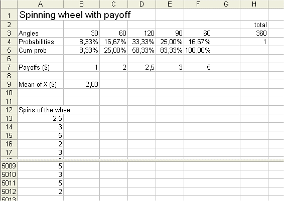
E(X) = $1 * 8,33% + $2 * 16,67% + $2,5 * 33,33% + $3 * 25% + $5 * 16,67%
= $2,83

By the way the above figure also gives the results of 5000 spins of the wheel. Are we interested in these results to evaluate the mean of X ?
Answer : No.
Since we know all the underlying probabilities of X, thanks to the very simple wheel that we know entirely, the additional knowledge of a past history of outcomes of X is of no use.
What is the variance of X ?
The variance of X is defined as the expectation of the squared deviation of X around its mean.
Here there are five possible squared deviations :
| 5 possible squared deviations | 3,36 | 0,69 | 0,11 | 0,03 | 4,69 |
The first one is (1-2,83...)2, the second one is (2-2,83...)2, etc.
The variance of X is 1,22 (technically, the units here are "squared dollars")
and the standard deviation of X is $1,11
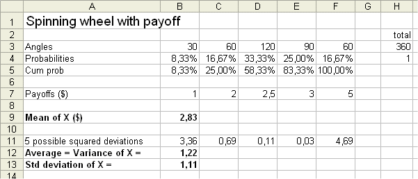
This measure of the spread, the standard deviation, here is $1,11. With some experience one can read off the payoffs and their probabilities that this result seems ok.
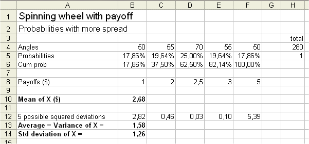
The spread depends upon the possible payoffs of course, and also upon their probabilities. If we keep the same payoffs, but we "spread" the probabilities more (like jam on a slice of bread), we will get a wider std deviation.
case 2 : we don't know the underlying distribution
Now comes a case that is closer to real life situations : we have a random generating device that produces outcomes, but we don't have access to the device itself. All we have is a series of past outcomes.
(To make life simple, suppose we still know the possible outcomes. But we don't know their probabilities.)
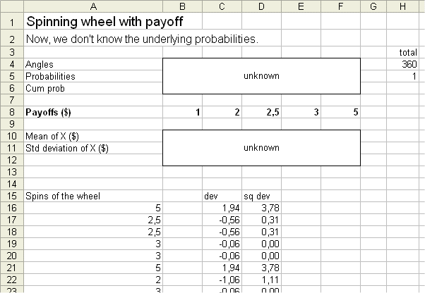
Now we definitely are interested in past outcomes to estimate the probabilities of each outcomes, estimate the mean of X, and estimate the variance and the std dev of X.
Two cases arise : either we have a very large past history, in which case we are sort of back to the case where we know everything, or we know a reasonable number of past outcomes, say 25 past outcomes. In this second case we make our estimations as common sense suggests.
Here is a series of 25 outcomes of X :
| Spins of the wheel | |
| 1 | 2,5 |
| 2 | 2,5 |
| 3 | 3 |
| 4 | 5 |
| 5 | 3 |
| 6 | 1 |
| 7 | 2 |
| 8 | 2,5 |
| 9 | 3 |
| 10 | 3 |
| 11 | 5 |
| 12 | 2,5 |
| 13 | 1 |
| 14 | 3 |
| 15 | 2,5 |
| 16 | 3 |
| 17 | 2,5 |
| 18 | 2,5 |
| 19 | 3 |
| 20 | 2,5 |
| 21 | 3 |
| 22 | 2,5 |
| 23 | 3 |
| 24 | 3 |
| 25 | 2,5 |
Counts :
$1 is counted 2 times
$2 is counted 1 time
$2,5 is counted 10 times
$3 is counted 10 times
$5 is counted 2 times
(We check that the total of counts is 25.)
So Pr{X=$1} is estimated to be 2/25=8%, etc.
The mean of X is estimated to be
$1*8% + $2*4% + $2,5*40% + $3*40% + $5*8% = $2,76
(It can be also calculated as the simple average of the 25 outcomes. It is exactly the same calculation.)
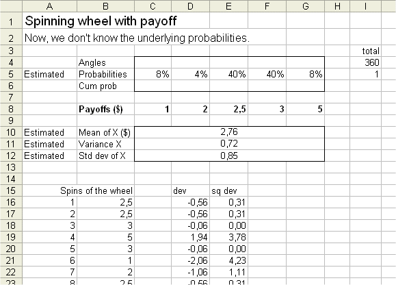
The variance is estimated in the same natural way. We take the estimated mean to put in the formula for the variance.
estimated variance of X = 0,72
and estimated std dev of X = $0,85
A note on estimation : because the estimated variance uses an estimated mean that is already "adjusted" to our outcomes, it yields an estimated figure for the variance that, on average (if we redo a large number of times this estimation procedure with a new set of 25 outcomes), is a bit too small. It is what is called "a biased estimator" : its mean is not what it tries to estimate. If we want it to be unbiased, like most of your hand held calculators do, we must divide by 24 instead of 25 in the formula for the estimated variance.
By the way, to require an estimator to be unbiased is a "common sense" requirement, although no undisputable argument can be made for it, since anyway our estimate is wrong :-) . And it turns out that for certain optimisation problems, surprisingly enough, certain biased estimators are superior. (See : James Stein estimators.)
(Can be omitted in a first reading. Mandatory study resumes with the Polyzone project)
In Finance, one of our objectives can be viewed as estimating the future profitability of such and such investment. Estimating parameters is, with testing whether a hypothesis seems correct or not, one on the central objectives of Statistics.
Two schools are in opposition on this problem :
The Bayesian view is harder to defend from an epistemological viewpoint. And it has not proved more efficient to make money.
The Frequentist school is not exempt of paradoxes too. For instance, here is the table of possible values of X and Y, giving the probabiliities of any couple of values :
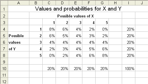
The construction of a confidence interval for the mean of X, given that Y = 3, leads to weird results. Since the outcome of Y belongs to (1,3) the likely mean of X is small, but since the outcome of Y belongs to (3,5) the likely mean of X is big.
In real life situations, we never know exactly what is all the relevant information (Y = something) we should take into account to estimate parameters concerning X (for instance the future profitability of such and such security).
A large American chemical producer, based on its superior competitive position and technology, wanted to invest into a new plant, in the United-States, to produce a chemical commodity called "Polyzone" to serve the European market. The project was forecast to be able to produce positive cash flows for ten years.
The financial analysts, in the Finance and the Accounting depts of the firm, began to "crunch numbers" to establish a budget for the project.
And, to compute the NPV of the cash flows they obtained, they used a discounting factor which was "the profitability of "main stream" securities in the chemical industry in the stock market". They chose r = 8%.
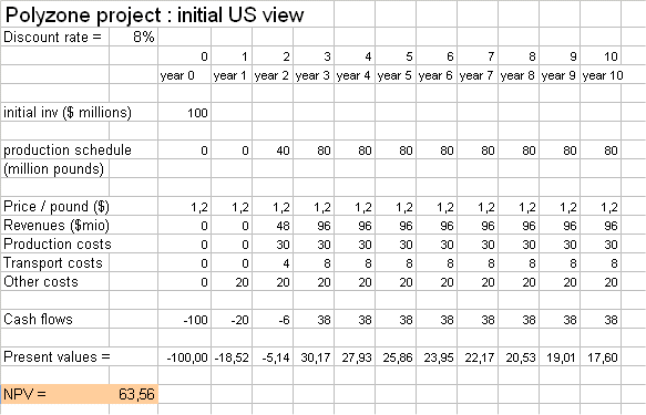
The project has an NPV of +63.56 million dollars, so they thought that this is a good investment.
This was until they realized, with the help of consultants, that when they begin to sell this product in Europe, it will attract local competition. It lead to a revision of their hypothesis concerning the selling price.
It may take a few years, during which they are alone as a supplier, but after a while there will be European competitors as well to sell Polyzone to the European market.
Pursuing this simplified analysis, the law of supply and demand will push the prices downward until the project ceases to be attractive to a new European entrant.
European entrants have a somewhat different budget for the "Polyzone project" : they don't have the transportation costs across the Atlantic ocean. (It is the line "transport costs" above). Then a European competitor contemplating entering into this business, at the price of $1,2 per lb, will have the following budget, and NPV :
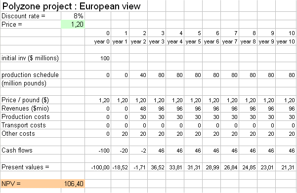
It will look great to a potential European competitor ! This will attract competition in Europe, from local producers, and it will lower the selling price from $1,2/lb to a figure that makes the NPV no longer attractive (i.e. zero).
This is attained for a price of $0,952 /lb. (Use the goal seek tool, on the Polyzone Excel document on the website, to find it.)
Therefore it is more realistic to forecast that, if the American producer builds the plant and begins to sell to Europe, it will be able to maintain a price of $1,2/lb for a few years, but then the price will decrease and stabilize around 0,95.
Here is, therefore, a more sober budget of the Polyzone project for the US firm :
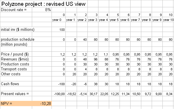
It is no longer an attractive project !
The US firm should not invest into the Polyzone project at the current level of prices, costs, and volumes it anticipates.
This quick analysis can be developed : it suggests that, if the US firm still wants to make the investment, it should either take measures to increase its volume of sales in Europe, or perhaps work more on the production process to reduce the production costs.
Here is a last budget, for the US firm, with lower production costs :
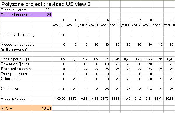
As we see, if the US producer can reduce its production costs to 25 million dollars per year (they don't depend upon the volume, because it is a large "process" production : the costs are essentially the team of people tending the machines, and other fixed costs), then the project becomes interesting again.
(By the way : to reduce the production cost is an investment in R&D that ought to be analyzed with a DCF analysis...)
"Monte-Carlo methods" is the name given to a family of astute uses of randomness to solve mathematical problems that are difficult to solve using standard techniques. Stan Ulam is credited with having invented these methods.
Here is an example : we have a disk quadrant inscribed into the unit square
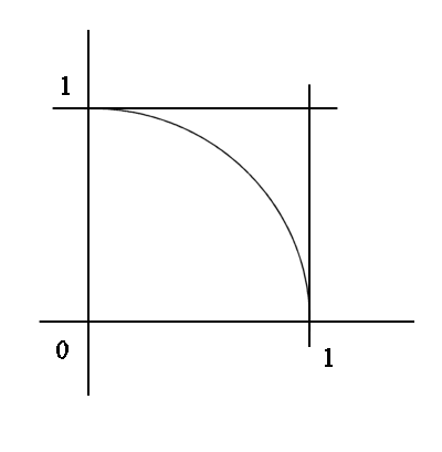
The surface area of the square is 1.
Suppose we want to evaluate the surface area of the quadrant. It is not too hard using geometry, but let's assume it is a difficult problem, and let's use a "Monte-Carlo method". It was given the name "Monte-Carlo method" because Monte-Carlo it is a beautiful city on the French riviera, famous for its casinos, that is places where we play with money and randomness.

The technique is this : "throw" a large number of random points, uniformly distributed, onto the square, and count how many fall into the circle.
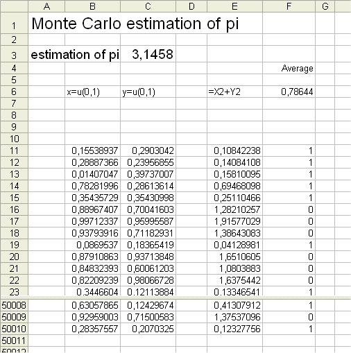
To generate, in a spreadsheet, a random point, uniformly distributed over the unit square, use the coordinates : x =rand() and y =rand() (in French this function is =alea() )
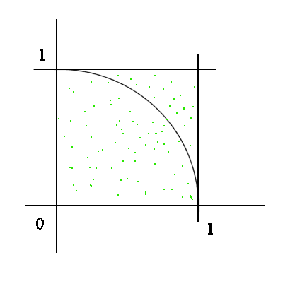
and check whether x2 + y2 is greater or less than 1 (Pythagoras theorem. See also : biography of Pythagoras). In the table below we generated, with Excel, 50 000 random dots, and we counted "one" each time it fell within the circle.
The proportion of dots within the quadrant is 78,64%, so the area of the quadrant is estimated to be 0,78644. And therefore the area of the whole disk is estimated to be four times as much, that is = 3,1458, which should not surprise us too much, since as we know the exact measure of the surface area of the full disk is Pi (it is in fact the definition of Pi.) And, from other non-Monte-Carlo methods, we can get Pi = 3,14159... Pi is a number that has fascinated mathematicians for more than two thousand years. References : 1 and 2. For instance :
Pi / 4 = 1 -1/3 + 1/5 - 1/7 + 1/9 - ......
(Some people still work on Pi, example. They do this not so much because there is much new to say on Pi, although..., but because they hope that the tools they design will be useful elsewhere.)
This method, in more elaborate situations, has proved very useful. It was refined, among other people, by Feynman and Kac. It is related to mathematical results, concerning the behavior of random walks, that play an important role in Finance. See for instance Ito's lemma.
Ito processes, also called Wiener processes, also called Levy processes, also called Brownian motion, also called Bachelier processes, because all these people studied them, are the mathematical representation of "things" that go randomly from one step to the next. Prices of securities seem to be adequately modeled, on reasonably short periods of time, by this type of random process.
(Examples of research on the subject. Remember : all it takes to be familiar with all this is practice. Those of you who want to go into Finance will study these subjects more deeply.)
IRR is the extension of the concept of profitability to a situation where profitability, as we are familiar with it, no longer applies.
Let's start with the situation where profitabilitiy is the natural concept we are familiar with :
Consider a security S with a price today of 80€, and an expected cash flow in one year of 115€.
Then, as everybody knows, the profit of S will be 35€, and therefore the profitability of S will be 35/80 = 43,75%. Fine !
The slightly more surprising fact is what happens when we apply a DCF analysis to S. Let's compute the NPV, with a discount rate r, of investing into S. We shall do the calculation for a series of discount rates r, so we shall get a result that is "a funtion of r". There will be a value for r=10%, a value for r=20%, etc.
What is the NPV of S for r=10% ?
Well, we discount the future cash flow by 10% : 115/(1+10%)=104,55 and we subtract the initial cash flow (that is the price) : - 80€. So the result is NPV(S;10%)=24,55€
Let's do it again for r=20% : NPV(S;20%) = - 80 + 115/(1+20%) = 15,83€
We keep on with a sequence of increasing r. When NPV(S;r) reaches zero, the value of r at that figure is called the IRR of S.
The slightly surprising fact is this : the NPV will become zero exactly when r reaches the profitability of S ! Let's check : NPV(S;43,75%) = - 80 + 115/(1+43,75%) = 0€. So the IRR of S is its profitability.
Secondly, let's look at a case where the usual concept of profitability no longer applies. Here is an investment I :
C0=80, C1=40, C2=50, C3=20
Now the usual concept of profitability ( (future money - today's money) / today's money ) no longer applies. It would be quite mistaken to say : "oh ! the profitability is (40+50+20-80)/80=37,5%"
(In fact, in particular, this mistaken measure would make no difference between I and for instance J=[C0=80, C1=110], which is obviously better !)
But here the concept of IRR still applies.
Let's compute the NPV(I;r) for a series of increasing r, from 0% to 50 or 60%. Then the r for which NPV(I;r)=0 will be the IRR.
NPV(I;0%) = 30
NPV(I;10%) = 12,71
NPV(I;20%) = -0,37
NPV(I;30%) = -10,54
So we know that the IRR is between 10% and 20%, close to 20%.
Let's try 15% : NPV(I;15%) = 5,74
Let's try 18% : NPV(I;18%)= 1,98
etc.
By one of the various methods presented in the past lessons, we get IRR(I)= 19,7%
So, here, this 19,7% is also called the "profitability of I". It it the definition of "profitability" in this situation.
By the way, "Internal rate of return" is another name for "internal profitability".
Risk and opportunity cost of capital :
There again there are two cases : the simple case of a security with one cash flow in one year, and the case of an investment with several cash flows in the future.
Case of a security S : we said that S has the same risk pattern as another security T, iff E(X)/sd(X) = E(Y)/sd(Y), where X is the random value of S in one year, and Y is the random value of T in one year. (No reference to prices today here.)
Then, if T has a price PT on the stock market, then T has a profitability rT.
This rT is also the opportunity cost of S.
And the maximum price PS we should be willing to offer for S, if we stick to the rule of Finance "For the same expected future cash flow, pay a higher price for the less risky security", is PS = E(X)/(1+rT).
It requires some care to be shown, and MBA textbooks usually are not clear or not careful enough in explaning this. Here is an example of outrageous explanations, dating from the time when Finance was a cookbook of recipes with no justifications except that they produced tasty cakes.
Then, all these ideas extend to the case of an investment with a stream of cash flows. There again, some care must be used in specifying the probabilistic model, for the cash flows of I, we use.
In this review lesson, let's not go into all the details again (go to lesson 5 part a, section on "Risk pattern and risk of an investment", for the details of the model). Let's just say this : the set of future cash flows of an investment I has the same risk pattern as securities traded in the stock market, in the same industry, in the same specific activity.
Let's call rI the profitability of these securities. Then rI is the opportunity cost of capital of I.
Just like for S (when we have identified T), the maximum price (i.e. cash flow C0) someone should be willing to pay for I today is the Present Value of the set of future cash flows discounted with the opportunity cost of capital of I. They are computed as this :
PV(C1; rI) = C1/(1+rI)
PV(C2; rI) = C2/(1+rI)2
PV(C3; rI) = C3/(1+rI)3
etc.
Each future cash flow is discounted with (1+rI)n where n is the number of years in the future Cn will appears. And the present value of the set of cash flows is the sum of the individual PV's.
If for us this is higher than the C0 we must invest initially, we are in a lucky situation : the NPV of I for us is positive. In theory, we can earn this money (and possibly more) right now, by "selling the investment" to somebody else.
Example : let's take again the investment I above (C0=80, C1=40, C2=50, C3=20). Suppose the profitability of securities traded in the stock market and with the same risk pattern as I is 12%. Then the NPV(I;opportunity cost of I)=9,81. It is positive, so I is a good investment.
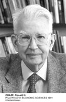
Ronald Coase (born in 1910) is a very interesting economist, for remarkable ideas on firms that he elaborated in the Thirties. I strongly advise you to read what he had to say on the subject. The gist is this : If the liberal system of free give and take, according to economic players' willingness, is the most efficient system, why firms internally don't function on this model ?
Another fun point about him is this : "Ronald Coase is an unusual economist for the twentieth century, and highly unusual for a Nobel Prize winner (he won in 1991). First, his writings are sparse. In a sixty-year career he wrote only about a dozen significant papers—and very few insignificant ones. Second, he uses little or no mathematics, disdaining what he calls "blackboard economics." Yet his impact on economics has been profound. That impact stems almost entirely from two of his articles, one of which was published when he was twenty seven. The other was published twenty-three years later."
Digression 2 : The objectives of Economics :
The objectives of Economics are
Since the end of the Ancient Régime, two centuries ago, the economic workings of most modern societies is based on the production and exchange of work to buy and consume goods and services, produced by work within firms. This is done via the medium of money and credit (a subtle form of money) to operate exchanges. And the banking system plays an important role in this too.
Classical Economics, following Adam Smith, says that this system works best when left to itself ("laissez faire, laissez passer"). The law of supply and demand via the "Invisible Hand", described by Smith, always takes care of filling out lacks, and moderating excessive increases. But everybody can feel that this theory, despite its intuitive attractiveness, is simplistic and mistaken. Complex dynamic systems are rarely optimal and stable. For those who like theorems (in a simplified setting though) there is the result of Sonnenschein-Mantel-Debreu that establishes the fallacy of Smith reasoning. The end word will be given in some future by nonlinear mathematics. See for instance the book Thinking in complexity by Klaus Mainzer.
Governments can act on two levers to influence and try to correct these workings :
But money is an elusive concept. Probably some concept of "money + credit" will turn out to be a better measure of the exchange capacity of each economic actor. Sometimes having more money gives more purchasing power, and sometimes the value of money gets corrupted. Why ? The reasons are many : for instance there may not be much to buy, or the power of some economic players to set the value of what they sell may be excessive (OPEC...). The "value of money" is essentially set in each private exchange. And, in a transaction, each actor has his own set of personal values, including that of money. Public control over "the value of money" is limited. It is a complex "intensity parameter" in the complex economic system.
Firms invest to grow and produce more wealth. They do that by trying to maximise profit. But profit too is an elusive concept. Classically, it is analyzed as the remuneration of risky capital. And probability theory is used to study this remuneration (the profitability of securities and investment that we will study all year long).
One aspect of the complexity of the system is this : firms are naturally encouraged to increase their productivity. This means producing the same output with less work, and therefore with less expenditures to buy work (mind you, this involves the value of money...). But work is the way consumers get their money, that enable them to buy goods... So productivity is not a panacea. Countries then distinguish between competitive industries (for instance, the automotive industry in Japan) and sheltered industries (for instance, the retail distribution sector in Japan), and say that what matters is the productivity and competitiveness of competitive industries... But this essentially mercantilist reasoning just moves the paradox from a domestic setting to an international setting...
So more work, most likely in the direction of nonlinear mathematical modeling, is necessary to understand how to achieve prosperity and fairness. And today's world is definitely in need of new economic views.
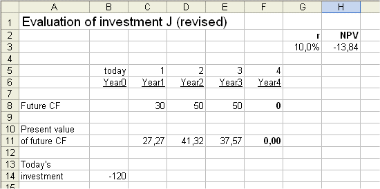
In the notes for lesson 5 part b, handed out this week, there is a mistake in the discounted cash flow analysis of investment J. The investment J was presented as having one initial cash flow to be spent C0 (=120 million €), and then four future cash flows produced C1=30, C2=50, C3=50 and C4=10.
But then all the DCF analysis was carried out without taking into account C4, which is equivalent to having C4=0.
So for instance it the NPV of J for r=10% was computed as -13.84 million €, which is definitely not true for the J with its four above future cash flows. The correct answer is NPV (J ; 10%) = -7.01
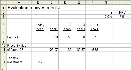
All the analyses and results presented last time become correct when we omit C4 (which is equivalent to setting it to 0). Then for instance the NPV (revised J ; 10%) = -13.84
