Wednesday January 5th 2005
Finance : eleventh lecture (part one)
Joint random variables and portfolios of securities
Introduction
Review of one random variable
Profitabilities are more interesting than prices
Standard financial model
Intuition
Work on one random variable
Percentages in finance
Back to X that can take three values
Position of X on the risk-return graph
Work on a second random variable
Position of Y on the risk-return graph
Admissible securities
Let's create an inadmissible security
Today's topic is the study of two random variables produced in the same experiment E. They will display their random variability "jointly". This study is a prerequisite to study investments into portfolios of securities, and their optimisation.
When we have $1000 to invest into the stock market, we usually don't want to invest it all into one security. We prefer to select several securities S, T, U, etc. and split our money into these securities. It is an application of the proverb : "Don't put all your eggs into the same basket". For instance we will invest $300 into S and $700 into T. This is called "investing into a portfolio made of 30% of S and 70% of T".
We need to study how our portfolio will perform according to the performance of each security. As far as the expectation of profitability is concerned, intuition readily gives a reasonable result, but the risk of our portfolio is less intuitive - we shall see this.
Securities in the market don't behave independently. Even though they display randomness, when the market is bullish they tend to all move upward, and when the market is bearish they tend to all decrease.
If securities in the stock market behaved purely independently of each other we could beat the rule that say that to make an investment more profitable, on average, than the risk free rate we must accept the possibility to loose money. Indeed we would select a collection of say 100 independent securities all yielding 10% average profitability, each with some risk. Then we would split our money into one hundred parts and invest into the one hundred securities. This would still yield 10% profitability, and with just about zero variability. This is unfortunately not possible :-)
(It is an application of the following fact : if we are asked to estimate the result of one throw of a die, no particular guess is good ; but if we are asked to estimate the average of one hundred throws of a die, we know that 3,5 will be a very good guess.)
Review of one random variable :
Remember : the concept of an experiment E was introduced to model the random behavior of one random variable, for instance the value X of a security S next year, or the profitability R of this security next year. If we bought our security S, today, for a price P, and next year S will have a value X, then R = (X - P)/P.
Ideally we want to find securities with high average profitability and low variability.
S may be a stock, for instance General Electric stock.

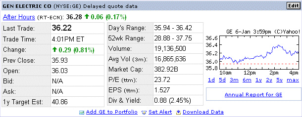
The price P today is $36.22. The value in one year is called X. We don't know the actual figure that it will be ; it is a random variable. X will have an outcome x. May be x will be $40, may be more. This would be nice for us. May be it will be less than the price today. At any rate it is not a sure figure, like would be investing into a short term US Treasury bond, which would have next year the price paid today times (1 + r0), where r0 is the risk free interest rate in the US. Last October r0 was 1.75%. Now, in early January 2005, it is 2.25%. It is Alan Greenspan and his advisors who decide the risk free rate in the US.
To have an average profitability higher than the risk free rate we must accept a risk, that is we must accept the possibility to loose money.
(A little bit of theory for those who will want to go deeper into Finance (it can be skipped) : Randomness produces an instance of the experiment E. It is called "an elementary event" attached to E, and it is denoted ω. The set of all possible elementary events for E is denoted Ω. Any subset of Ω has a probability, that is any possible event A attached to the experiment E has a probability Pr{A}. Sometimes the collection of events A's of E is denoted F. So you will see in textbooks a "full probabilistic model" denoted : (Ω, F, Pr). If there is no confusion between probability and price, it is denoted (Ω, F, P).
To the instance ω of E corresponds an "outcome" of the random variable X, denoted x = X(ω). In other words, in a more elaborate presentation of the theory of probability and finance, a random variable X is a function from Ω (the "universe of instances of E") to some space of outcomes taken by X (it can be numbers, it can be colours, it can be other characters, countries, sexes, etc.) ; earlier we have denoted them : a1, a2, ... ap ; most often the possible values of X are the real numbers.
And events concerning outcomes of X (for instance {X ≥ $40}) correspond to events in F. This looks heavy handed, and indeed we shall not use this formalism, but we should know that in more advanced finance this turns out to be the clearest and most convenient way to study the behavior of securities - in particular, options.)
We think of waiting from today until next year like "producing an instance of the experiment E related to the evolution of GE price between today and next year". Buying a GE stock and waiting one year is a bit like playing a game of chance throwing a die.
Suppose that from past observations of GE prices we figure out that, next year, X, the random value of GE, can take the following possible values, with the following probabilities :
| Value of GE stock in one year | |||||||||
| Possible outcomes | $25 | $30 | $35 | $40 | $45 | $50 | $55 | ||
| Probabilities | 5% | 10% | 20% | 30% | 20% | 10% | 5% | ||
Note that here we transformed a continuous random variable into a discrete approximation. We could model GE stock next year more finely, if we preferred ; or we could even model it with a continuous RV, but then we would need a bit of Calculus to make calculations on it.
Continuous RV are more complicated to deal with at first, but in more advanced finance they are simpler than discrete RV.
Continuous RV can always be approximated by discrete RV : we just round them off like done above.
Then the event A = {value of GE stock in one year is greater than or equal to $40} has a probability of 65%.
We can even compute the expectation of X and the standard deviation of X :
E(X) = $40
σ(X) = $7,25
If we prefer to work on the profitability of our purchase of one stock of GE, then R next year can take the following values with the following probabilities :
| Profitability of GE stock in one year | |||||||||
| Possible outcomes | -31,0% | -17,2% | -3,4% | 10,4% | 24,2% | 38,0% | 51,8% | ||
| Probabilities | 5% | 10% | 20% | 30% | 20% | 10% | 5% | ||
E(R) = 10,4%
σ(R) = 20%
Here I'm making up a classroom example of what GE stock may be in one year. In a later lesson we shall see which actual estimates the market has for E(R) and σ(R) for GE.
Remember, GE stock is more profitable on average than a US TB (in my example E(R) = 10,4% instead of 2,25%), but there is a "price" for this : GE stock is more risky. Buying GE stock will earn us on average 10,4% (instead of 2,25%), but we may "draw a bad number" in the experiment E "waiting one year", and we may loose money next year - which is not possible with a US Treasury bond.
Profitabilities are more interesting than prices :
If we have some money to invest in the stock market, say $1000, and we have decided to devote about 1/3 of that sum to GE, it does not matter to us whether GE stock today costs $36 or $63, or anything (with a reasonable price). If GE quotes $36, we shall buy 9 stocks, and if GE quotes $63 we shall buy 5 stocks. What matters is the expected profitability of GE and its risk.
In an efficient market all securities (or even portfolios) yielding the same return (for instance 10% average return) have more or less the same risk (to be precise, we mean "the risk related to the market, and that cannot be eliminated by averaging" ; more on this in lesson 13), otherwise there would be good ones, and there would be bad ones that nobody would want.
The above model for securities, their random behavior, and the random profitability to get from investing into them, is the standard model in Finance.
The characteristics of GE stock, computed above, are rGE = 10,4% and σGE = 20% (classroom example). Stocks are represented on the figure below :
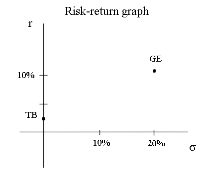
Everybody working in the stock market is somewhat familiar with this model and this graph. And investments funds make more and more use of professionals trained in mathematical finance, that develop this model.
There are other models but they are more controversial and so far they haven't proved to be better.
Intuition tells us, correctly, that if we invest $1000 into two securities S and T, where S has average profitability rS and T has average profitability rT, and the split of our money is α into S and (1- α) into T, then the profitability of our investment will be the weighted average
α rS + (1 - α) rT
Numerical example : we invest $300 into S, and $700 into T. S has average profitability 10% and T has average profitability 5%, then the average profitability of our investment is
30% x 10% + 70% x 5% = 6,5%
In other words, in one year, on average we will have $1065.
But what about the risk ? (That is the standard deviation of the random profitability.)
Suppose S has risk 25% and T has risk 15%. What is the risk of our "portfolio" ? Intuition does not give us the answer.
In fact we need to know more about S and T : we need to know their joint probabilistic behavior.
And we will discover that a combination of investments into S and T, plus possibly keeping some money (or borrowing some money), will be superior to either S or T !
This was clearly understood and described only in the 1950's. Harry Markowitz got the Nobel prize, in 1990, for his work of the 50's on this subject.
Let's consider a random variable X that can take three values a1, a2 and a3, with probabilities 25%, 35% and 40%.
Suppose X is the profitability of a security. (In order to avoid too many notations, I no longer use R for the profitability.)
a1 = -5%
a2 = 5%
a3 = 10%
What is the expectation of X ? And what is the standard deviation of X ?
In finance, percentages occur in two instances :
It is somewhat unfortunate - and the words even sound alike ! - but there is not much to do (except teach in another language...).
Remember : a percentage notation means nothing more than "divided by 100".
So 3% = 0,03
square root of 3% = square root of 0,03 = 0,1732...
square root of u is the number z, such that
z times z = u
Sometimes it is easier not to carry percentages all over the place. But sometimes percentages are more suggestive.
(When you see in some textbooks "... times 100%", it means nothing more than "... multiplied by 1". It is introduced to try to be clearer, but it is a moot question whether it is indeed.)
Back to X than can take three values :
X is a random profitability. It can take three values. It is an arch-simplification of real life. It is a classroom example to make calculations on random variables, compute expected profitability and risk. (In fact most profitability random variables, in real life, have more or less bell shape distributions, unlike this example. But for learning purposes it may be better to be more general.)
The expectation of X is by definition :
E(X) = a1 Pr{X = a1} + a2 Pr{X = a2} + a3 Pr{X = a3}
We saw that this weighted average is a natural definition because it is the value to which the simple average of many many outcomes of X, in a large number of replications of the experiment producing X, tends to.
Indeed if we produce 10 000 outcomes of X : x1, x2, x3, ...., x10000 , then the simple average of the xi's will be very close to E(X) as defined above. The reason is that in the 10000 xi's,
about 10 000 times Pr{X = a1} will be equal to a1,
about 10 000 times Pr{X = a2} will be equal to a2,
about 10 000 times Pr{X = a3} will be equal to a3,
We verified this fact several times, in earlier lessons, with the random number generator of Excel. If you are still unsure of this fact, construct X with the random number generator of Excel and check it by yourself. (Its deep justification is pure counting, but this does not concern us. Intuition about randomness is better.)
Here is an example of a few outcomes of X (in the third row) :

The cells of the first row contain "= RAND()", and the third row is defined as shown in the formula window.
So here E(X) = 4,5%
| Values | Prob | products |
| -5% | 25% | -0,012500 |
| 5% | 35% | 0,017500 |
| 10% | 40% | 0,040000 |
| Mean value | 4,50% |
The risk of a security is defined as the standard deviation of its profitability.
The standard deviation of a random variable is the square root of its variance.
The variance of a RV is the expected value of its squared deviation :
the square deviation of X can take three values
| Values | Prob | products | squared dev | |
| -5% | 25% | -0,012500 | 0,009025 | |
| 5% | 35% | 0,017500 | 0,000025 | |
| 10% | 40% | 0,040000 | 0,003025 | |
| Mean value | 4,50% |
The expected value of this squared deviation is
sq_dev1 . Pr{X = a1} + sq_dev2 . Pr{X = a2} + sq_dev2 . Pr{X = a2} = 0,003475
| Values | Prob | products | squared dev | products | |
| -5% | 25% | -0,012500 | 0,009025 | 0,002256 | |
| 5% | 35% | 0,017500 | 0,000025 | 0,000009 | |
| 10% | 40% | 0,040000 | 0,003025 | 0,001210 | |
| Mean value | 4,50% | Variance | 0,003475 | ||
| sd | 5,89% |
0,003475 is the same thing as 0,3475%
and the square root of this number is 5,89%.
Position of X on the risk-return graph :
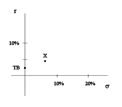
If, avoiding too heavy notations, we assimilate X and its security we can draw X on the risk-return graph :
Work on a second random variable :
Here is a second random variable, Y, representing the profitability of a second security :
| Y | ||
| Values | Prob | |
| b1 | -5% | 31% |
| b2 | 15% | 37% |
| b3 | 25% | 32% |
As we can readily see, Y has a higher mean value than X, and also has more variability.
Calculations confirm this :
E(Y) = b1 Pr{Y = b1} + b2 Pr{Y = b2} + b3 Pr{Y = b3}
= -5% x 31% + 15% x 37% + 25% x 32%
= 12%
And sd(Y) = 12,12%
Details :
| Values | Prob | products | squared dev | products | |
| -5% | 31% | -0,015500 | 0,0289 | 0,008959 | |
| 15% | 37% | 0,055500 | 0,0009 | 0,000333 | |
| 25% | 32% | 0,080000 | 0,0169 | 0,005408 | |
| Mean value | 12,00% | Variance | 0,014700 | ||
| sd | 12,12% |
Position of Y on the risk-return graph :
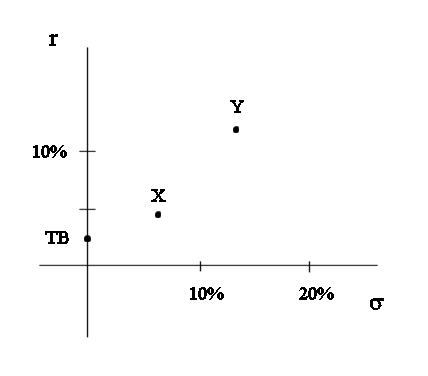
We note that if we only have the choice between Treasury bonds, X and Y, then no investment is bad.
All of them are "admissible".
An investment would be "inadmissible" if there was another one that, at the same time, was less risky and was more profitable.
Let's create an inadmissible security :
An inadmissible security Z would be one with a low profitability and a high risk.
Let's create a Z with profitability around that of X, and risk around that of Y. Then clearly it will not be admissible.
Here are some figures for Z :
| Values | Prob | products | squared dev | products | |
| -15% | 33,333% | -0,050000 | 0,04694444 | 0,01564815 | |
| 10% | 33,333% | 0,033333 | 0,00111111 | 0,00037037 | |
| 25% | 33,333% | 0,083333 | 0,03361111 | 0,0112037 | |
| Mean value | 6,67% | Variance | 0,027222 | ||
| sd | 16,50% |
E(Z) = 6,7%
and risk of Z : σ(Z) = 16,5%
The position of Z on the risk-return graph is this :
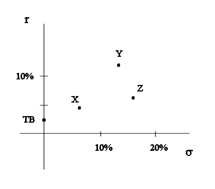
Z would be admissible if compared only to TB and X, but it is no longer admissible if Y is another possibility of investment. Indeed from the point of view of finance people Y is superior to Z : it has less risk and more average profitability. So Z is to be discarded as a possible investment.
(Remember : the rule of finance people is not that of gamblers, who attach value to the possibility of a high gain, disregarding its low probability. So gamblers might still like Z. But this is a course in finance, not in playing the loto...)