Wednesday January 12th 2005
Finance : twelfth lecture (part two)
Portfolios of securities (cont'd)
A small
program computing correlation in swarms of points
A portfolio made of some X and some Y
Expectation and Variance of Z =
αX + (1 - α)Y
For some value of α, Z makes X inadmissible !
Admissible portfolios
Introduction of Treasury bonds into possible portfolios
The straight line from TB and tangent to admissible portfolios
Conclusion about the capital market portfolio M
A small program computing correlation in swarms of points
With Excel we can easily create a small program which computes the correlation of the components of points in a swarm :
we position numbers (representing numbers of points, or dots) in an array. These points have the coordinates indicated along the sides, as follows
| Y | |||||
| 10% | 0 | 0 | 1 | 1 | |
| 5% | 1 | 3 | 3 | 2 | |
| 0% | 2 | 3 | 3 | 0 | |
| -5% | 1 | 1 | 0 | 0 | |
| X | -10% | 0% | 10% | 20% |
then the program transforms them into percentages
| Y | |||||
| 10% | 0,00% | 0,00% | 4,76% | 4,76% | |
| 5% | 4,76% | 14,29% | 14,29% | 9,52% | |
| 0% | 9,52% | 14,29% | 14,29% | 0,00% | |
| -5% | 4,76% | 4,76% | 0,00% | 0,00% | |
| X | -10% | 0% | 10% | 20% |
and computes the interesting numbers
E(X) = 4,3%
σ(X) = 9,5%
E(Y) = 2,6%
σ(Y) = 4,0%
Correlation (X, Y) = 52%
Let's use this program with a few examples of "swarms" :
| Y | |||||
| 10% | 0 | 0 | 0 | 1 | |
| 5% | 0 | 0 | 3 | 0 | |
| 0% | 0 | 2 | 0 | 0 | |
| -5% | 1 | 0 | 0 | 0 | |
| X | -10% | 0% | 10% | 20% |
Correlation = +1
because of the strict positive linear relationship.
| Y | |||||
| 10% | 1 | 2 | 3 | 1 | |
| 5% | 2 | 4 | 6 | 2 | |
| 0% | 1 | 2 | 3 | 1 | |
| -5% | 0 | 0 | 0 | 0 | |
| X | -10% | 0% | 10% | 20% |
Correlation = 0
because we can see the independence (the rows, and the columns, are proportionnal).
| Y | |||||
| 10% | 0 | 1 | 1 | 0 | |
| 5% | 1 | 3 | 2 | 1 | |
| 0% | 1 | 3 | 2 | 1 | |
| -5% | 0 | 1 | 1 | 0 | |
| X | -10% | 0 | 10% | 20% |
Another case of Correlation = 0. (Here the RV's are not independent, but almost : having information on Y does not give much information on X. In fact here we have a discrete approximation of a joint Gaussian distribution.)
| Y | |||||
| 10% | 1 | 0 | 0 | 0 | |
| 5% | 2 | 2 | 1 | 0 | |
| 0% | 1 | 3 | 3 | 2 | |
| -5% | 0 | 1 | 3 | 2 | |
| X | -10% | 0% | 10% | 20% |
Correlation = -59%
because we have a negative link : when X is large, Y tends to be small.
A portfolio made of some X and some Y :
We are now ready to study the performance of a portfolio made of some X and some Y.
Suppose that the security corresponding to X sells for $33,3 and the security corresponding to Y sells for $50, then investing in a "50%-50%" portfolio means buying 15 securities X and 10 securities Y. In other words, what matters to define the percentages in our portfolio is the money spent on each security, not the number of securities.
We shall look at a portfolio Z made of α X and (1 - α) Y, where α is a percentage between 0 and 100%.
We want to know the Expectation of Z and the Variance (and standard deviation) of Z.
Expectation and Variance of Z = αX + (1 - α)Y :
In order not to be too heavy in terms of notation we have assimilated securities and their random future profitabilities X and Y. The advantage is lightness ; the drawback is that we have to be careful about what we mean. When we talk of Z = α X + (1 - α) Y, we mean that "Z is the profitability of a security made of the proportion α of our money into X and (1 - α) into Y".
The expectation of Z is straightforward :
E(Z) = α E(X) + (1 - α) E(Y)
Let's take some specific random profitabilities for X and Y :
| Y | ||||||||||||||
| 50% | ||||||||||||||
| 45% | 1% | |||||||||||||
| 40% | 1% | 1% | 1% | 1% | ||||||||||
| 35% | 1% | 2% | 2% | 2% | 1% | 1% | ||||||||
| 30% | 1% | 2% | 2% | 2% | 2% | 2% | 1% | |||||||
| 25% | 1% | 3% | 4% | 4% | 3% | 1% | ||||||||
| 20% | 1% | 1% | 3% | 4% | 4% | 3% | 1% | |||||||
| 15% | 1% | 2% | 3% | 3% | 3% | 2% | 1% | |||||||
| 10% | 1% | 1% | 2% | 2% | 2% | 2% | 1% | |||||||
| 5% | 1% | 1% | 1% | 2% | 2% | 1% | 1% | |||||||
| 0% | 1% | 1% | 1% | 1% | 1% | |||||||||
| -5% | 1% | |||||||||||||
| -10% | ||||||||||||||
| X | -20% | -15% | -10% | -5% | 0% | 5% | 10% | 15% | 20% | 25% | 30% | 35% | 40% |
Calculations show that E(X) = 11,1% and E(Y) = 20%.
E(Z) is a simple linear combination of E(X) and E(Y). For instance, if α = 20%, then
E(Z) = 20% x 11,1% + 80% x 20% = 18,22%
For the variance of Z, things are not quite as straightforward. The formula is :
Var(Z) = α2Var(X) + 2α(1 - α)Covar(X, Y) + (1 - α)2Var(Y)
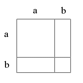
In fact this formula is less complicated than it looks. It is just a variety of the well-known formula for the square of a sum :
(a + b)2 = a2 + 2ab + b2
This last fact has a very simple geometric interpretation :

If we look at the area of the complete square (of side a + b), we readily see that it is the sum of the area of the square of side a, plus the area of the smaller square of side b, plus twice the rectangle of sides a x b.
In the example above
Var(X) = 0.00763
Var(Y) = 0.01198
and Covar(X, Y) = 0.00423
Then, still with α = 20%,
Var(Z) = 0.04 x 0.00763 + 2 x 0.2 x 0.8 x 0.00423 + 0.64 x 0.01198 = 0.00932
and σ(Z) = 9,7%
For some value of α , Z makes X inadmissible !
Before showing this surprising fact, let's position X and Y on the risk return graph :
E(X) = 11,1%, σ(X) = 8,7%
E(Y) = 20%, σ(Y) = 10,9%
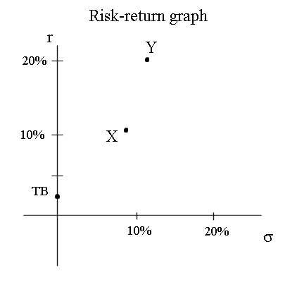
(Be careful that the standard deviation is on the abscissa, and the average profitability on the ordinate axis.)
With these data for X and Y, let's compute E(Z) and σ(Z) when α = 70%.
E(Z) = 13,8%, and
Var(Z) = 0.49 x 0.00763 + 2 x 0.7 x 0.3 x 0.00423 + 0.09 x 0.01198 = 0.00932 = 0.0065935
and, therefore, σ(Z) = 8.1%
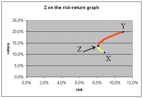
So we see that, when α = 70%, Z is more profitable that X and has less risk. That is, Z makes X inadmissible.
The complete curve of Z when α varies from 100% to 0% is this :
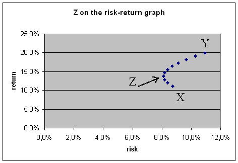
α = 100% is the bottom point (it is simply X), and α = 0% is the top-right point (it is simply Y).
The admissible portfolios are those on the red part of the curve (between Z and Y), and those that are inadmissible are on the yellow part of the curve (from X to Z) :
Introduction of Treasury bonds into possible portfolios :
If we can make portfolios mixing up securities and TB, then we can do even better than Z70% or the other admissible portfolios shown above.
The idea is simple, and the calculations even simpler : consider a security with a random profitability U, average profitability E(U) and risk σ(U).
For instance E(U) = 17% and σ(U) = 9%, then consider a simple mix of U and Treasury bonds : for instance V = 50%U + 50%TB.
Then not only E(V) is halfway between E(U) and 2,25%, but also σ(V) is halfway between σ(U) and 0%. The trick is that Var(TB) = 0% and Covariance(U, TB) = 0.
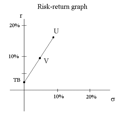
The consequence is that, if we are allowed to include TB in our portfolios, we can move between any portfolio already achievable and TB on a straight line.
The next, and final, trick is that we shall fit a line going through the TB point and tangent to the admissible portfolios.
The straight line from TB and tangent to admissible portfolios
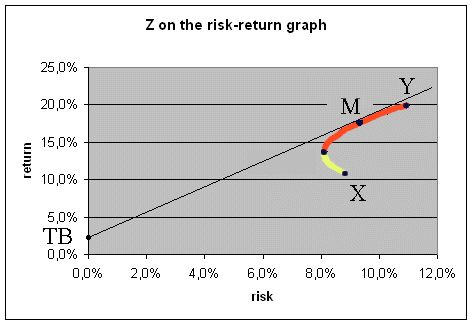
The straight line going through the Treasury bonds and tangent to the curve of admissible portfolios touches these admissible portfolios at a point M.
This point M, that corresponds to a portfolio called "the capital market portfolio", is very interesting :
Conclusion about the capital market portfolio M
With the above securities X and Y, M is roughly at α = 30%.
Then if we have the choice between any combination of X, Y and TB, the only good portfolios are a mix of the capital market portfolio M and TB. (With our data, M = 30%X + 70%Y.)
This is a first illustration of the following central fact in the Standard model of Finance : in order to make an efficient investment into the stock market we only have to select the level of risk we want to bear, and then make our investment into the mix of TB and M that achieves this risk. We don't have to worry about the individual behavior of all the securities in the stock market.
Put more bluntly : spending a lot of time reading carefully, in the newspaper, the performance of each stock in the stock market, in order to make optimal portfolio investments, is just a waste of time. Just invest your money one part into TB and the other part into the capital market portfolio.
Next time, we shall briefly see how this is developed into the fulfledged Capital Asset Pricing Model theory (CAPM).