
Wednesday January 19th 2005
Finance : thirteenth lecture (part one)
Portfolios of securities (3)
Introduction
Basics and notations
A paradox
More on US Treasury bonds
Portfolio of two securities :
behavior when the correlation changes
Exercise
Relationship between simple averages and weighted averages
Back to the exercise
Computation of the covariance and the correlation
Geometrical interpretation
With this lecture we finish up our brief introductory study to the Capital Asset Pricing Model (CAPM), that explains how securities in a stock market are positioned in the risk-return graph (and in another "twin graph" we shall meet) and how to optimise investment into portfolios made of several securities. Next lecture will be devoted to exercises to review the whole semester, and the following one is the final examination for this first semester of theoretical finance.
The CAPM was developed in the mid-sixties, after more than ten years of intense work to apply probability theory to the analysis of the behavior of securities. Together with the theory of option pricing, it is the crown achievement of what, nowadays, may be called "classical financial analysis of the stock market". Even though it does not work perfectly well, it provides a useful framework to approach investing into securities. After all, we use all the time models which we know don't work very well and yet are useful : for instance our representation of the way people function and behave.
The fulfledged notations about one security are these :
S : the name of the security. Today, for instance, we shall study Coca-Cola.
P : its price today. Coca-Cola price, as at the 22 January 2005, is $41.
We can obtain information on Coca-Cola from the website of the company (Coca-Cola Company) :

or from Yahoo Finance (or any other financial site) :
X : its price in one year. Of course, we don't know it today.
R : the resulting profitability it will have had, retrospectively, in one year. R = (X - P)/P
r : the expected value E(R) of that profitability
σ : the standard deviation σ(R)
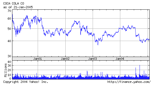
From the past data plotted above we can see that the past prices and profitabilities of Coca-Cola (read directly from the graph) were approximately :
Jan 2000 : P = $65
Jan 2001 : P = $60 and R = -7,7% ( = (65 - 60)/65 )
Jan 2002 : P = $48 and R = -20%
Jan 2003 : P = $45 and R = -6,3%
Jan 2004 : P = $50 and R = + 11,1%
Jan 2005 : P = $41 and R = -18%
The standard model says that the series of values of R is a random walk with certain probabilistic parameters r (=expectation of R) and σ (=standard deviation of R).
(When a firm distributes dividends, to be accurate we must add the dividends paid to calculate the profitability, from one year to the next, of investing into the stock of the firm. At any rate, in our subsequent study, we shall only look at profitabilities ((value in one year - price today) / price today), not at prices.)
But you may think that you know better what are the causes of the movements of Coca-Cola price and of its profitability.
Indeed a basic approach to explaining the price of a security is this : it is the discounted value of all the future dividends the market (that is, the investors, the analysts, etc.) expects. So when bad news hit the firm, the market revises downward its estimates ; and when good news come from the firm or about the firm, the market revises its estimates upward.
From the above graph we also see that there was a lot of trading on Coca-Cola in September 2004. And the price went from $45 to $40. Some bad news must have reached the market concerning Coca-Cola. Or, just, some more or less "irrational" review of Coca-Cola price took place. At any rate, many stockholders thought it was time to sell ; and many others thought that at the price offered Coca-Cola was a good buy. (In fact, in September, the firm released information saying that, at the end of 2004, it would probably not meet its 2004 forecast results, established earlier in the year.)
When there is no confusion we call S, P, X and r : "Coca-Cola".
If for two securities, for instance Coca-Cola and Compaq (before it merged with Hewlett-Packard) we have, from one source or another, good estimates of the probabilistic parameters r and σ, of each, we can position them on the risk-return graph as follows :
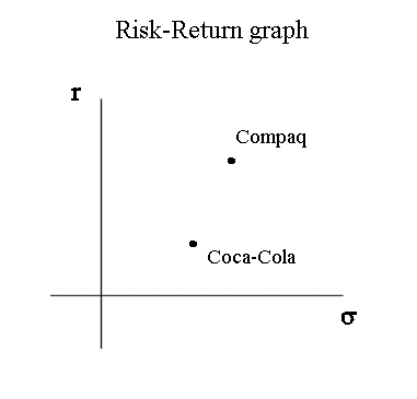
It may seem as a paradox to position Coca-Cola on the risk-return graph at some positive ordinate height, when we see that the last five yearly profitabilities are : -7,7%, -20%, -6,3%, +11,1%, -18%.
But remember that r is the return of Coca-Cola expected by the market at its current price. For example, right now the current price of Coca-Cola is $41. Obviously the market expects that Coca-Cola value next year (dividend + reselling price) will be higher, otherwise nobody would want to pay today $41 for it.
In other words, the price of a security, at any date, results from a market adjustment, so that its expected profitability (in the future !) is positive and is in line with what the market wants for the level of risk of the security.
Not only does the market expect the value of Coca-Cola next year to be more than $41 dollars, but it must be significantly more (depending on its risk), because even no risk securities (that is US Treasury bonds) yield 2,25% (on a yearly basis) at the moment.
When we have dollars and don't know what to do with them, the least we can do is invest them into US TB (with all the caveats about this "common sense reasoning"). They are supposed to be "safe" and they yield something. China has a lot of US TB, between $150 and $200 billions as at January 2005, resulting from a large positive trade balance with the United-States and other countries (see table of US foreign bond holders in November 2004).
The exact monetary and financial status of these holdings is an important question that we shall study next semester in our course in International finance. To begin building our intuition we may ask ourselves the following questions :
Note that China is becoming edgy about its US bonds holdings, and so is Japan. China shows intention of curtailing its US bonds holdings, and increases at the same time "its foreign exchange reserves". But in which currencies ? How to get paid when you run a trade surplus ? Credit, Paper promises, Bonds, Currencies, Gold, Stocks, Buildings in Manhattan, other Investments, etc. ? We shall study all these : they are elements constructing the very important national accounting document called "the Balance of Payments".
Note too that China and the other countries holding large exchange reserves have the power to very significantly influence the exchange rate between currencies. To some extent the dollar/euro exchange rate fluctuations that we witness these days are the result of China policy vis-à-vis its dollar denominated holdings.
As you know there is, at present, in 2005, a big problem in the world (financial and not financial) that results from the very large US trade deficit with the rest of the world, that the United-States have built over the last 20 years, and which they pay for with Treasury bonds issued by their government. In 2005, the US trade deficit will be around $600 billion. The US TB themselves compensate the US budget deficit : that is why we talk about the "twin deficits" of the United-States.
Portfolio of two securities : behavior when the correlation changes
Let's consider a portfolio Z constructed with two securities X and Y, with a percentage α of X and the percentage (1 - α) of Y.
(X, Y and Z here represent the profitabilities of the three financial objects.)
We saw that
E(Z) = αE(X) + (1 - α) E(Y)
and
Var(Z) = α2 Var(X) + 2 α (1 - α) Covar(X, Y) + (1 - α)2 Var(Y)
We can rewrite the same formula, where Covar(X, Y) is replaced by
Corr(X, Y) σ(X) σ(Y)
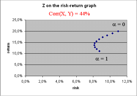
Consider the following numerical example :
E(X) = 11.1%, σ(X) = 8.7%
E(Y) = 20%, σ(Y) = 10.9%
Corr(X, Y) = 44%
Then the curve of the various portfolios Z when α goes from 0 to 1 is this :
Now comes the interesting points.
1) What would the curve have been if the two securities X and Y had been perfectly positively correlated ?
Calculations yield this
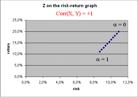
It can be seen readily from the formula for Var(Z) when Corr(X, Y) = 1. Indeed, then
Var(Z) = [α σ(X) + (1 - α) σ(Y) ]2
therefore the points ( σ(Z), E(Z) ), when α changes, move on a straight line.
2) The case when Corr(X, Y) = -1 is even more interesting :
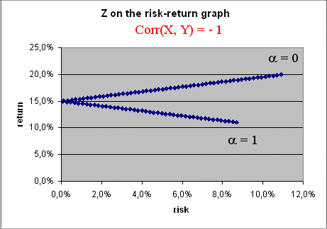
Conclusion : if we could find two securities X and Y perfectly negatively correlated, we could construct a portfolio Z with zero risk and a profitability somewhere between that of X and that of Y. Of course this is impossible in real life : the stock market does not offer such possibility. Otherwise everybody would invest his money in such a way and make large sure amounts of money.
This has a very concrete meaning :
We shall extend these results to a more general form. And we shall even see that, in an ideal market, securities available for investment are always positively correlated. But before this, let's do more exercises to build up our familiarity with the joint behavior of random variables.
(There are many websites that present this material with their own style. Here are three :
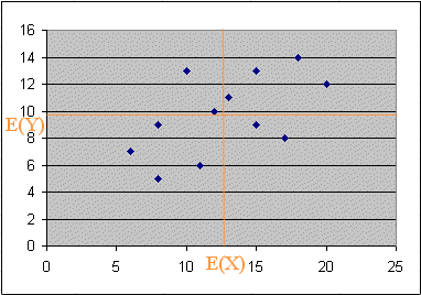
Suppose we have twelve measurements of two variables (X, Y) produced jointly in an experiment E. They are represented here :
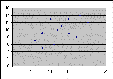
These dots (or points) are twelve outcomes of (X, Y) :
(x1, y1), (x2, y2), ..... (x12, y12)
This is the extension to two dimensions of considering a series of outcomes of one random variable.
The numerical values are these :
| values of X | values of Y |
| 15 | 9 |
| 8 | 9 |
| 11 | 6 |
| 13 | 11 |
| 6 | 7 |
| 8 | 5 |
| 17 | 8 |
| 18 | 14 |
| 10 | 13 |
| 12 | 10 |
| 20 | 12 |
| 15 | 13 |
Let's compute the estimated values of E(X), σ(X), E(Y), σ(Y), covar(X, Y) and corr(X, Y) :
the estimation of E(X), which in a heavy handed way we could denote Est_E(X), but that we shall just denote E(X) is the simple average of the xi's :
E(X) = (15 + 8 + 11 + ... + 20 + 15) / 12 = 12.75
Relationship between simple averages and weighted averages :
Why do we take the simple average of the twelve outcomes of X ?
Because here we do not have the probabilities of each possible outcome (we don't even know what actually is the set of all possible outcomes of X). So we cannot work with the probabilities of each possible outcome and with the theoretical formula for E(X).
But what we do is equivalent to estimating the probabilities of possible outcomes of X and using the theoretical formula.
Indeed, to understand this better, let's round off X to values in the middle of three intervals :
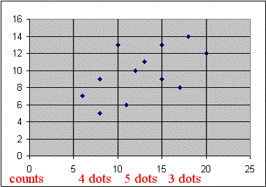
X is not far from a random variable "Xround" that took
4 times the value 7.5
5 times the value 12.5
3 times the value 17.5
This random variable has a histogram :
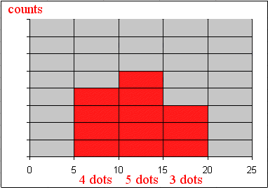
Then we can estimate the probabilities of each value of Xround :
Pr{ Xround = 7.5 } = 4/12 = 33%
Pr{ Xround = 12.5 } = 5/12 = 42%
Pr{ Xround = 17.5 } = 3/12 = 25%
And we can apply to Xround the theoretical formula for an expectation :
E(Xround) = 7.5 x 33% + 12.5 x 42% + 17.5 x 25% = 12.1
This is, of course, not exactly equal to the simple average of the xi's, since we rounded them off, and we tended to lower them a bit (those on the lines were counted in the left interval).
In other words a weighted average is like a simple average where we first have done some grouping of data.
To compute the variance of X we need to compute the twelve squared deviations of X around its mean :
| squared deviations |
| of X |
| 5,06 |
| 22,56 |
| 3,06 |
| 0,06 |
| 45,56 |
| 22,56 |
| 18,06 |
| 27,56 |
| 7,56 |
| 0,56 |
| 52,56 |
| 5,06 |
The simple average of these twelve squared deviations is the estimated variance of X. The result is Var(X) = 17.52
And the standard deviation of X is the square root of the variance : σ(X) = 4.19
The same calculations on Y yield :
E(Y) = 9.75
σ(Y) = 2.80
With some practice you will become able to check from the scattergram of (X, Y) that these figures seem correct :

| E(X) = | 12,75 | sd (X) = | 4,19 |
| E(Y) = | 9,75 | sd (Y) = | 2,80 |
Computation of the covariance and the correlation :
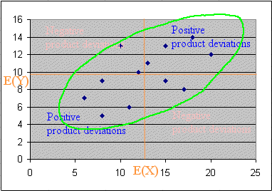
The covariance of X and Y is defined as the expectation of the products of deviations :
Covar(X, Y) = E{ [ X - E(X) ] times [ Y - E(Y) ] }
From our twelve outcomes of products of deviations
(x1 - 12,75)(y1 - 9,75), (x2 - 12,75)(y2 - 9,75), .... (x12 - 12,75)(y12 - 9,75)
we shall compute the simple average.
Here again this is an estimation that is equivalent to computing the theoretical expectation if we had the probabilities of each possible pair of outcomes.
| values of X | values of Y | Product |
| of deviations | ||
| 15 | 9 | -1,6875 |
| 8 | 9 | 3,5625 |
| 11 | 6 | 6,5625 |
| 13 | 11 | 0,3125 |
| 6 | 7 | 18,5625 |
| 8 | 5 | 22,5625 |
| 17 | 8 | -7,4375 |
| 18 | 14 | 22,3125 |
| 10 | 13 | -8,9375 |
| 12 | 10 | -0,1875 |
| 20 | 12 | 16,3125 |
| 15 | 13 | 7,3125 |
Average of the products of deviations = Covar(X, Y) = 6.60
There is an important geometric fact to notice : the covariance being the sum of products of deviations, when the points form an elongated swarm slanted along the upper-right direction, there will be more products that are positive (and large) than there will be negative products. Therefore the covariance is going to be positive. And the correlation too.
Finally the correlation is
Corr(X, Y) = Covar(X, Y) / (σ(X) σ(Y)) = 6,60 / (4,19 x 2,80) = 56,3%
So, as expected, X and Y are positively correlated.
It can be shown with some a bit more advanced algebra, or geometry, that a correlation coefficient must always be between -1 and +1.
Break time