Finance with a review of accounting

Random variables, expectation, wheel of chance

Random variables

We are all familiar with situations, in real life, where a measurement of some value, or some quantity, or some feature, can be made, and this measurement is not fixed. By "the measurement is not fixed", we mean this :

• the "situation" can be reproduced

• the same value, or quantity, or feature, can be measured again

• the result of the measurement will not be the same

On top of this, if we reproduce the situation many times, there will be some stability in the pattern displayed by the various measurements.

Vocabulary :

• the "situation" will be called : the experiment

• the value, or quantity, or feature, the measurement of which varies, will be called a random variable

• each measurement, for each replication of the experiment, will be called an outcome of the random variable

If you think it bizarre to speak of something which "changes all the time", note that we can talk about objects, irrespective of where they are. A random variable X is "something" the measurement of which changes when we measure it from replication to replication of an experiment.

We have an "object-oriented", in a 3-D space + one time line like the real numbers, perception of daily life. It is this "object-oriented perception" which troubled so much XVIIIth century philosophers with the question "What remains permanent in a piece of wax which can change place, form, color, firmness, become gazeous, etc. ?"  It is at the same time very convenient to go about our daily business, eat, sleep, have fun, but it is sometimes a hindrance for a deeper understanding of the world. For instance, most people are troubled by the fact that the question "What was there 20 billion years ago?" is not meaningful in Physics. Another example is this one: we grow up accustomed to just about every phenomenon having a cause (except precisely in randomness - this disturbed even Einstein who exclaimed "Gott würfelt nicht!"), therefore getting older we are troubled because this universe we live in appears to have no cause, and some of us stick a cause on it in order to feel comfortable. Then this explaining cause fulfills many other purposes like justifying revolting ways of life.

One of the beauties of probabilities is this : if you set up an experiment and reproduce it many many times, and each time measure the same random variable, you will observe some stable pattern in the series of outcomes of the random variable. If you telephone a friend, describe the experiment and the random variable to be measured, and suggest him or her to reproduce the experiment and the measurement a long series of instances too, your friend will certainly not get the same series of outcomes, but he or she will observe the emergence of the same pattern !

Examples

Dice

It seems that dice are the first example in history, beginning in Antiquity, where man began to understand randomness : something that changes from replication to replication with no exact prediction possible, and yet with a long term pattern in a series of replications. If I throw a die, I will get an outcome which is a number in the set {1, 2, 3, 4, 5, 6}. These six numbers are the six possible outcomes of the throw of a die. The experiment here is "throw a die once". The random variable is "result of one throw". The possible outcomes are the finite set {1, 2, 3, 4, 5, or 6}.

Notation, the set of possible outcomes of a random variable which can take a finite number of values is usually denoted

set of possible outcomes of X = {a₁, a₂, a₃, ..., a_p}

(We use this heavy handed notation in order to generalise easily to other situations, like the wheel of chance that we shall study next. Of course, here p = 6, and the a_i's are simply enough the first six integers.)

Suppose I throw the die 20 times, I will get twenty outcomes. Usually they are denoted

x₁, x₂, x₃, ... x₂₀

Here is one series of 20 throws :

Here is another series of 20 throws :

It is quite important not to mix up the set of a_i's and the series of x_i's.

These series of 20 throws are quite interesting. Any given series of 20 throws has the same probability as any other, and therefore these probabilities are very small, because there are 3 656 158 440 062 980 different possible such series.

But in these almost 4 million of billions series, most of them have more or less the same proportion of each possible a_i. For instance, those where one of the a_i's is missing are rare (less than 3% of them). Those where one of the a_i's appears more than half of the time are very rare. Etc. Whereas those where the proportions of each a_i's are not far from 1/6 are very frequent. In other words, when we throw a die many times, we get roughly each outcome one sixth of the time.

Here is another illustration of this perhaps strange looking  fact : toss a coin three times ; there are 8 possible resulting series :

HHH

HHT

HTH

HTT

THH

THT

TTH

TTT

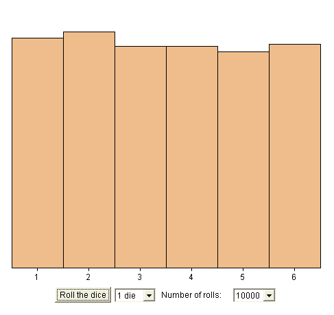
Note, in these 8 possible results, that most of them contain "head" and "tail". That is, forcing a bit things, "most of them display experimental proportions close to 50-50" !

As a consequence, if we measure probabilities from a long experimental series, we have a good chance to get experimental probabilities close to the true ones.

Check : throw one die 10 000 times (instead of 20 times), using the following java simulation https://www.stat.sc.edu/~west/javahtml/CLT.html

Let's count how many times we got each possible outcome. Here is the result :

If we accept that symmetry leads to the equiprobability of the faces, and that highly probable events will appear much more often than events with small probabilities, then the fact that we usually observe an even distribution of experimental results is only an arithmetical result in numbering. (See explanation below.)

Wheel of chance

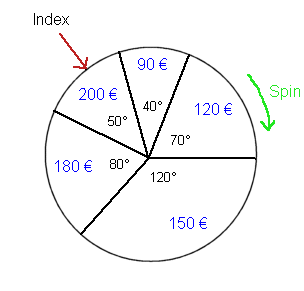
Consider the following device : a wheel that can turn freely around its axle, and an index fixed on the frame of the device (not on the wheel). The wheel is divided into five angles, and each angle shows a sum of money.

It is a wheel of chance to play a game : we spin the wheel once, and we win the payoff shown in blue by the index.

With this example we get one step closer to the financial situations in the stock market and in physical investments we are eventually interested in.

Here the experiment is "spin the wheel once". The random variable (RV) is "the payoff shown by the index".

The set of possible outcomes is

Now the five possible outcomes are no longer "equiprobable" like the six faces of the die were. But, if the wheel is well balanced, we know the probabilities from the angles.

Here is a first series of 20 spins of the wheel (x₁, x₂, x₃, ... , x₂₀) :

Here is a second series :

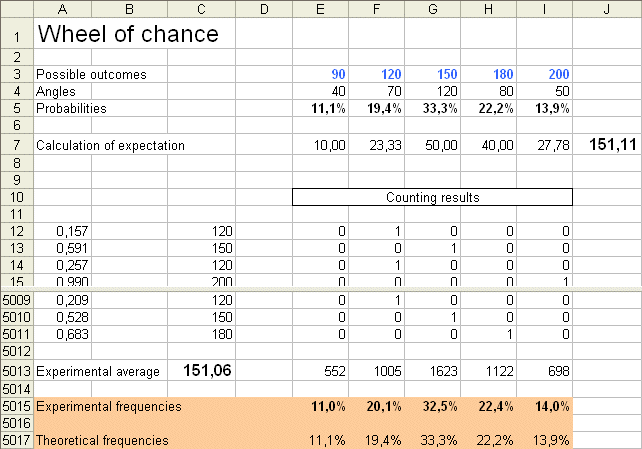
If we produce a very long series of outcomes of payoff, we know that we will get experimental frequencies, for the five a_i's, close to the theoretical frequencies, which are

40/360,   70/360,   120/360,   80/360,   50/360

We can check this with an excel sheet which simulates the spin of the wheel 5000 times : virtual wheel of chance.

Here is one result, after 5000 spins :

As we can see, the approximations are very good. Just like for the die, this is not magic, it is a purely arithmetical result in numbering : most possible experimental distributions of frequencies are close to the theoretical one. So we got one of them.

To understand this purely arithmetical result, think of flipping a coin four times. When we flip a coin 4 times we have 16 possible series of heads and tails. You can easily count that we get (4 heads , 0 tails) once, (3 heads, 1 tail) 4 times, (2, 2) 6 times, (1,3) 4 times, and (0,4) only once. With other types of random variables it is the same arithmetical fact at work.

Indeed, in the same way, think of our wheel of chance as made of 360 small sectors of 1 degree each. When we spin the wheel once, every sector gets the same chance (1/360) to come up, because of symmetry. When we spin the wheel 5000 times (like tossing the coin 4 times), we get one series of 5000 results, out of a gigantic number of possible series of 5000 results. It so happens (and can be shown) that most of these series display experimental frequencies close to the theoretical probabilities of the initial 5 sectors (just like, for the coin tossed 4 times, most of the possible series have experimental probabilities "close to" 50-50. Of course it would be more convincing with 10 or 20 tosses of the coin). So we got one series, and naturally enough it falls into the subset where the experimental frequencies are close to the theoretical ones (because so are most of them).

Therefore, the "law of large numbers", which states formally the above result, is nothing more than a result in arithmetic.

(Secondly the distribution of possible experimental averages around the theoretical average - see below - is bell shaped (with a rather narrow spread). For those of you interested in probabilities, this is " the Central Limit Theorem".)

An interesting question is : "How much are we willing to pay to play this game ?"

Are we willing to pay 50 € ?

- Sure ! The minimum gain is 90 €.

Are we willing to pay 250 € ?

- No.

Are we willing to pay 100 € ?

- It looks like a good deal.

What about 150 € ?

In fact the question boils down to : "What is the average value of the payoff ?" By "average payoff" we mean the average value of the possible payoffs, each of them weighted by its probability. We will come back to this question and the concept of expectation. But let's continue with examples first.

Light bulbs

Consider a manufacturing process producing light bulbs, all of them of the exact same model, that is, as identical as we can make them. We know that these light bulbs won't have exactly the same life time. If we select six of them for a statistical test of quality, we may get the following life times in hours (there are ways to make accelerated tests, that yield results which lead to the life times...) :

Here the experiment is "test one light bulb". The random variable is "the life time of the light bulb". The possible outcomes are no longer a finite set of numbers, it is the whole range { 0 hours, up to +∞ hours }. In this case, we say that the random variable is continuous, taking values in the positive real numbers.

Return of securities

I buy a security today, for instance one Air Liquide share. I pay 151,6 €. Suppose that, in one year from now, I sell it back and also receive a dividend : altogether I cash in, for instance, 180 €. To model this and make financial calculations, the standard tool in finance is probabilitiy theory.

Here the experiment is "buy one share of Air Liquide, wait one year, and sell it back (and get also the possible dividend)". Here the random variable we shall look at is the profitability of our operation : its outcome, in this instance, is (180 - 151,6) / 151,6 = 18,7%.

We could look at another random variable : the price itself. But we would run into a small technical problem : the prices from one year to the next are not independent from each other. Whereas the series of profitabilities are independent from each other. (More on this when we introduce the concept of independence, in probability : roughly speaking, two RV produced in the same experiment are independent if knowing the outcome of one does not give any extra information on the other on top of what we already know about the second one.)

Conclusion on the examples

We shall discover that probability theory is a very powerful tool to study various situations in real life where some values, quantities or features vary from one replication of the situation to another.

When using probability theory, one must be very clear "which experiment are we talking about ?" Without the experiment being clearly specified, we run into plenty of fuzziness and/or paradoxes. For instance, the question "Picking a person at random, what is the probability that this person is Chinese ?" is unclear. If the experiment is "pick at random equiprobably among all human beings", the probability is about 1/4. If the experiment is in this classroom, the probability is 1/50.

RV don't necessarily take numerical values. "Pick two socks at random in a drawer" is a random experiment, and the random variable of interest, "the pair of socks" we pick, is not numerical. Yet we can ask "Is it a pair of matching socks ?" But we cannot compute the average of a series of pairs of socks. In this finance course, however, we will only consider numerical random variables. Most of them will be profitabilities. This will unfortunately be a possible source of confusion, because we will talk about percentages which are probabilities, and about percentages which are profitabilities.

Bell shaped distributions

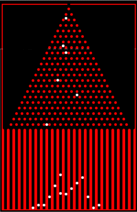
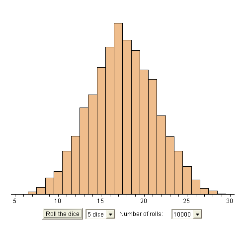
Most random variables we shall deal with will have a bell shape distribution (from the family of so-called "Normal distributions", or "Gaussian distributions"). This is a consequence of a result in probability : when we sum up many independent random variables (and none of them is dominant), the sum is a random variable which has a bell shape distribution.

Here are two examples :

1. Balls falling through a mesh of nails, and at each step they go either left or right (see illustration below). The distribution of ending positions can be viewed as the sum of many +1's (a turn right) and -1's (a turn left):

2. Summing up several dice. The experiment is "throw five dice together". The random variable is "the sum of the five results". Here is the experimental frequency distribution of results from reproducing the experiment 10 000 times (https://www.stat.sc.edu/~west/javahtml/CLT.html)

Bell shaped distributions are a family, depending on two parameters : one of them is the position of the middle of the bell on the abscissa ; the other is related to the width of the bell.

Classification of random situations

The random situations and variables we shall study in this course will fall into four categories, the consequence of two dichotomies :

1. we shall study random variables with a finite set of possible outcomes (like a die, or the wheel of chance above) ; and we shall study RV with a continuous set of possible outcomes (like profitabilities of securities, or future cash flows produced by investments)

2. there will be situations where we know everything about the RV : the set of possible outcomes, and the probabiliites ; and there will be situations where we only know one past series of outcomes.

This classification is quite important. Consider the first row (random variables having a finite set of possible outcomes). Suppose we look at a random variable X in the right (green) column : we don't know the "underlying distribution" of the RV, we don't know all the a_i's for sure, nor the probabilities, but we know a past series of outcomes of X (x₁, x₂, x₃, ..., x_n). Then these past data are very useful. And if n is large enough, it's as if we knew everything about X. Conversely, let's consider a random variable Y in the left (pink) column, about which we know everything, like for the wheel of chance above. In this case, knowing, on top of that, a past series of outcomes of Y is of no use.

In finance, we never know the "theoretical probabilities" driving the behavior of a given RV (i.e. we are never in the left column). But we usually have some past data at our disposal.

Expectation of a random variable

Let's focus again on the above wheel of chance :

a₁ = 90 €
a₂ = 120 €
a₃ = 150 €
a₄ = 180 €
a₅ = 200 €

We also know the probabilities of each outcome :

We already mentioned informally "the middle value" of a random variable. Now, let's define precisely what we mean :

By definition, the expectation of the random variable X is the weighted average of its possible values, weighted with their respective probabilities :

E(X) = a₁*Pr{X=a₁}+a₂*Pr{X=a₂}+a₃*Pr{X=a₃}+a₄*Pr{X=a₄}+a₅*Pr{X=a₅}

With our example the numerical calculations yield :

E(X) = 90€*11,1% + 120€*19,4% +150€*33,3% + 180€*22,2% + 200€*13,9% = 151,11€

This is the maximum price, to pay for the ticket to enter the game, which guarantees that in the long run we don't lose money. If we pay less, in the long run we earn money. If we pay more, in the long run we loose money.

The formula for the expectation of the random variable X may appear quite formidable at first. But we shall discover in a moment that in fact it is a very natural formula that we are all familiar with, perhaps without knowing.

Simple averages and weighted averages

Take two amounts of money, for instance $100 and $200.

The simple average of these two numbers is

($100 + $200) / 2 = $150

Now let's compute the weighted average of $100 and $200 with the weights 30% and 70%. It is, by definition :

$100*30% + $200*70% = $170

To figure out what is the natural meaning of this weighted average, one way is to realize that it is equivalent to the simple average of ten numbers, three of them being $100, and seven of them being $200.

(100 + 100 + 100 + 200 + 200 + 200 + 200 + 200 + 200 + 200) / 10 = 170

In other words, a weighted average "gives more importance", in the calculation of the average, to the elements with large weights.

That's exactly what randomness does in producing a series of outcomes of a random variable X. It will produce more often the possible outcomes with high probabilities, and less often those with low probabilities. Let's see what this means more precisely : if we reproduce the experiment producing an outcome of X (the above wheel of chance) a large number of times, say 10 000 times, we will get 10 000 numbers

x₁, x₂, x₃, x₄, ... ... ..., x₁₀₀₀₀

Remember : each of these x_i's is a number belonging to the collection of five numbers {90€, 120€, 150€, 180€, 200€}.

Question : In the series of 10 000 x_i's, what is the proportion of 90 ? (90 is the first possible outcome, which we called a₁)

Answer : If the series is very long - and here it is sufficiently long - the proportion of a₁'s is close to Pr { X = a₁ }= 11,1%. The same is true for the proportion of a₂'s, the proportion of a₃'s, of a₄'s and of a₅'s.

Therefore the simple average of the x_i's, which is (x₁ + x₂ + x₃ + x₄ + ... ... ...+ x₁₀₀₀₀ ) / 10 000, or equivalently

a₁* (actual frequency of a₁) + a₂ * (actual frequency of a₂) + ... + a₅ * (actual frequency of a₅),

is very close to the weighted average of the a_i's, weighted by their probabilities.

Summary : When n is large, the simple average of n outcomes of X is close to the expectation of X.

Thus, we see the origin of the formidable looking formula for the expectation of X (also called the mean of X). And we already checked this experimentally : in the above picture presenting the result of 5000 spins of the wheel, the theoretical mean is 151,11€ and the experimental mean (the simple average of the 5000 outcomes) is 151,06€.

This result, that may be surprising, is only a property of numbers. It is possible to chance on an experimental mean which is far away from the theoretical mean (it could be as low as 90€, or as high as 200€), but it is extremely unlikely.

Percentages which represent probabilities, and percentages which represent profitabilities

In Finance, unfortunately enough, we shall be lead to study formulas which mix up percentages representing probabilities, with percentages representing profitabilities.

Example : Suppose we pay P = 120€ to play the game with the above wheel of chance.

Question : What is the profitability of the game ?

Answer : It is a random variable - let's call it R - which has five possible outcomes :

r₁ =   (90 - 120) / 120 = -25%
r₂ = (120 - 120) / 120 =    0%
_r3 = (150 - 120) / 120 =  25%
_r4 = (180 - 120) / 120 =  50%
r₅ = (200 - 120) / 120 =  67%

Exercise : Compute the expected profitability of the game, using two methods.

Solution :

1. Method 1 : we compute the weighted average of the five r_i's, and we get 25,9%

2. Method 2 : we note that R = (X-120)/120 = (X/120) - 1 ; so E(R) = [ E(X) - 120 ] / 120 = (151,11 - 120)/120 = 25,9%

In other words, playing this game of chance, where we must pay 120€ at the beginning, has an expected profitability of about 26%.

This little example is not very far from what we do in the stock market : we purchase today a share of some firm, we pay P, and we expect to receive, in one year (selling back the share) a sum X.

When X is a sure sum, it is no longer a random variable (or, if you prefer, it is a random variable with no variability !), and, in that case, in the euro zone, we are ready to pay a price P = X / (1 + 4%) to buy today this security (4% is the risk free rate in late October 2007).

But if X, with the same expected value as above, has variability (and if, adds the CAPM theory, this variability is linked to the fundamental economic uncertainty of the market), then we only accept to pay less than E(X) / (1 + 4%) to purchase the security corresponding to X. The more variable is X, the less we will be willing to pay. That's why "junk bonds" were so cheap.

(Junk bonds are cheap - compared to their average pay-off -, and therefore have a high average profitability. Yet you cannot "beat" the market, average several junk bonds, maintain the average profitability of your portfolio, while reducing the variability of its profitability. That's one of the central results - in line with reality - of the Capital Asset Pricing Model. If we have time we shall construct computer models, using the software Flash, of stock market portfolios in order to understand precisely this phenomenon.)

The wheel of chance models somewhat the stock market :

The experiment E is : buy a ticket for the game and spin the wheel once -> buy one stock of Accor  (66.29 euros as of October 24th, 2007) and wait one year, and sell it back (and get the dividend too).

The random variable is the payoff of the game -> the value you get from the dividend and sale back of Accor's stock

The possible outcomes : a1, a2, ..., a5 -> all the possible values you can get after one year

A series of outcomes : the results of spinning the wheel many times -> think of reproducing the same year many times.

If investors were offered a sure payoff of 151.1 euros in one year, they would agree to pay around 145 euros today for this ticket. (Because the risk-free rate today is 4% in the euro zone).

But since the payoff only has an average of 151.1 euros, and has some variability they will be willing to pay less than 145 euros. Because they are risk-averse.

Gamblers may be quite willing to pay 170 euros to play the wheel of chance. Why ? Because they say : "I can gain 200 euros!"

To understand the gamblers, think of a situation where you have 170 euros in your pocket and, for some reason, you desperately need 200 euros. In that case you may accept to play the wheel of chance. Because the extra 30 euros has a utility for you that is much higher than what the money says. This question belongs to the paradox of Bernoulli and the theory of utility.

Go to lesson 7