Finance with a review of accounting

Distribution of probabilities, variance & standard deviation, simulations

Introduction

Last lecture, we began the study of simple probability theory and random variables, because we need this toolbox to study investments (financial or physical), their profitability, their risk, how to compare several investments, how to choose good ones. Today we shall continue with the study of one random variable produced in an experiment. Later in this course, we will study several random variables produced in the same experiment and the relationships they may show, in order to study portfolios of securities. Tomorrow we will begin studying the technique called "discounting". At the end of today's lecture we should feel at ease with the following concepts :

single random variables (discrete or continuous)
theoretical probabilities
simulation
past series of outcomes
histogram
theoretical mean / experimental mean
variability, defined by the variance and the standard deviation

Distribution of probabilities

A random variable X is always produced by an experiment E. Sometimes, this experiment is obvious and explicit, like throwing a die ; sometimes, it is only a mind concept, like when we talk about the probability that such and such government decision lead to less unemployement (we don't intend to reproduce many times the situation and count how many times unemployement was reduced...). In this course, we only deal with numerical random variables taking their values in the so-called real numbers. Some will be discrete and finite, some will be continuous.

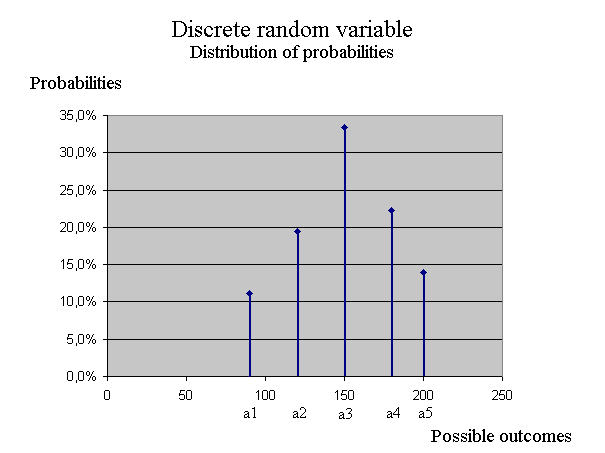
Discrete random variables

A discrete, and finite, random variable X can take only a finite number of possible values, which we denoted {a₁, a₂, a₃, ... a_p}. For each a_i, there is a probability p_i that the outcome of X be a_i. We use the notation

p_i = Pr { X = a_i }

so we have p₁ + p₂ + p₃ + ... + p_p = 1. (No relationship between p the probability, and p the index ; we just need notations.)

A possible representation of X is this :

We can check that the 5 probabilities add up to one :

Sometimes, these a_i's and these p_i's are entirely known to us. Sometimes, they are not, but we know a past series of outcomes of X, which enables us to know the a_i's and obtain approximations of the p_i's.

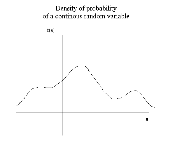
Continuous random variables

A continuous random variable X can take any value a in the set of all numbers. We run into a problem when we want - like we just did above - to represent its probabilities : for any value a, the probability that X be equal to a is zero. So instead of considering the numbers Pr { X = a }, which for any a is zero, we look at the local density of probability near any value a. The density of probability of X near a value a, is denoted f(a). It is a function of a. And, staying casual in our wording, it is defined as this :

where ε is small. If we step back and look at this formula, we see that it is definitely a "density" near a.

Densities are a very common concept, which we use all the time, may be without knowing. Any measurement defined as a ratio of a quantity by a distance, an area, a period of time, etc is a density. Examples :

• force per square meter : it is a pressure ; a large, heavy, but soft object resting on a floor may exert different pressures at different points.
• distance covered per hour : it is a speed ; a car going from Bordeaux to Clermont-Ferrand will have different speeds at different times.
• angle of a mountain road with the horizontal line : it is a slope ; the slope can change from place to place.
• flow of water from a faucet : it is a debit per second ; it may vary.

A density of probability is a function, and is represened like this :

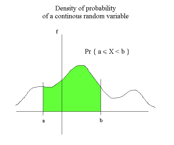
This is the very general possible picture of a density : a continuous line above zero, and such that the entire area beneath the curve is 1.

When we have the density f of a random variable, the probability that X be between any two values, a and b, is obtain by the area under the density curve between a and b.

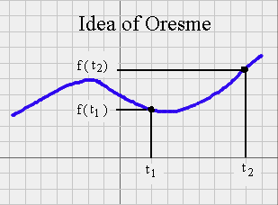
There are plenty of functions f for which, surprisingly enough, it is easy to compute the green area between any a and b. This is the mathematical technique called Calculus. We will not use calculus in this course.

Calculus was developed by Newton and Leibniz in the XVIIth century. (They spent a lot of time argueing who invented it first.) But some seminal ideas where already grasped by Nicolas Oresme in the XIVth century, that is at the end of the Middle Ages, before the Renaissance. Oresme understood that when we have a quantity f that depends upon another quantity t (for instance the speed of a horse that depends upon the time), it is possible to represent the relationship between the two quantities on a graph : we represent on a horizontal straight line the various times for which we know the speed ; for each time, we raise a point at a height corresponding to the speed at that time ; if we have plenty of points we get a curve. It was already fantastic to be able to give a graphical representation of a relationship. But, on top of this, Oresme understood that the area under the curve he obtained, between times t₁ and t₂, is equal to the distance covered by the horse.

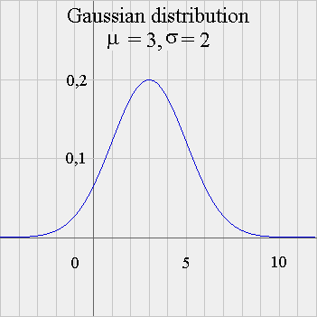
In finance most continuous random variables we meet are normally distributed (bell shape curves). A normal density depends on two parameters, denoted μ and σ. In other words, normal distributions are a family of curves, depending on two parameters.

The formula for the bell shape curve with parameters μ and σ is rather complicated. It is :

Here is the picture of f, for μ = 3 and σ = 2, with the scales on each axis, for once !, precisely represented :

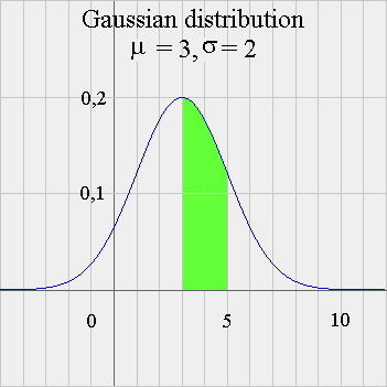
For instance, if X has such a density of probability, then Pr { 3 ≤ X < 5 } is the green area below :

Gaussian distributions (another name for "normal distribution", or "bell shaped" curves) have a complicated formula (see above). And it is not possible to come up with a simple mathematical formula for the area under the frequency curve between two points a and b. But with computers, this is no longer a problem : computers calculate very easily numerical values of all sorts of complicated formulas. For instance, when X is Gaussian ( μ = 3 and σ = 2 ), Pr { 3 ≤ X < 5 } = 0,342 = 34,2%. And, in fact, we can check on the picture that the area in green is a little more than 3 small rectangles (each of them has the area 1 x 0,1 = 0,1).

We already defined the expectation of a random variable X for a discrete random variable : E(X) = weighted average of the possible outcomes, weighted with their probabilities. And we saw that a long past series of outcomes of X will have a simple average very close to E(X).

All this can be extended to continuous RV. It requires a bit of Calculus, which we won't go into ; so we shall remain at an intuitive level. (For students interested in what exactly is Calculus, a brief introduction can be found here.) It is still true that a long past series of outcomes of X will have a simple average very close to E(X). In the case of a Gaussian random variable X, with parameters μ and σ, it turns out - not surprisingly - that E(X) = μ. And we shall see in a moment what is the geometric interpretation of σ.

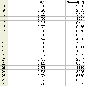
Simulations of random variables

With Excel - we already saw this - we can simulate random variables, that is we can "reproduce many times" an experiment E and produce outcomes of a random variable X, for which we have decided what is the theoretical distribution of probabilities (either discrete or continuous). For instance we can "produce" 20 outcomes of a normally distributed random variable with parameters μ = 3 and σ = 2. It is useful because, with this tool, we can put ourselves in the situation of having only a past series of outcomes, but also compare it with the theoretical characteristics which we have chosen for the random variable under study.

To do this, with Excel, we use the function RAND() (in French, ALEA() ) which produces random outcomes with a uniform distribution between 0 and 1. We get a series of 20 outcomes. And then to each of these outcomes we apply the function INVERSE NORMAL DISTRIBUTION (in French, LOI NORMALE INVERSE with the parameters μ = 3 and σ = 2). Here is a result (using the Excel sheet included in the folder of this lesson : Simulation_normal.xls) :

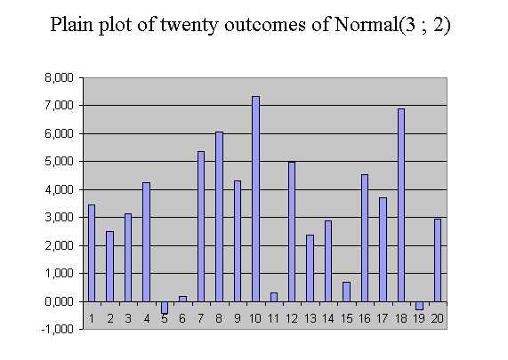
The twenty outcomes of Normal(3 ; 2) have an experimental mean of 3,257. This is not very far from 3, and it doesn't come as a surprise.

The twenty outcomes vary around 3 : the highest value is 7,331 and the smallest is -0,441. They have a certain variability for which we want to introduce a measure. It will be the variance of X that we shall define in a moment.

But before defining with a concept, and a formula, the variability of a random variable, let's us introduce the concepts of "plain plot of the data" and of "histogram".

Simulation of the sum of 8 uniform(0,1), to illustrate the convergence towards a bell shape distribution (Central Limit Theorem).

Plain plot of the data

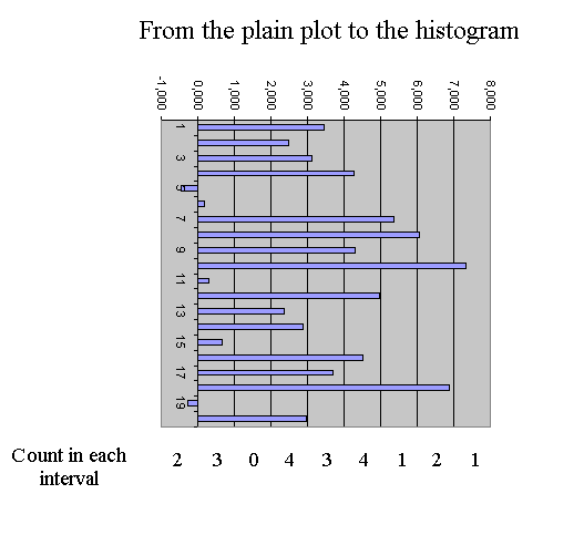
It is simply the plot of the series of data we have : on the abscissa, we position the ranks, and on the ordinate axis the values. With the above series of 20 outcomes of X normal (μ = 3 and σ = 2), it yields this :

Histogram of the data

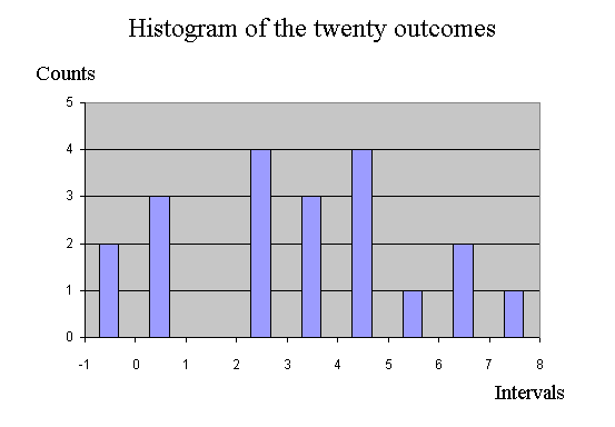
From the twenty outcomes of X produced above, there is another graph that is more interesting that the plain plot of the data : it is the histogram of the data. We will split the vertical axis into regular intervals, and count how many outcomes fell in each interval. So in truth there are many possible histograms, since we have to choose the intervals on the vertical axis. If they are too wide, all the data will fall in one interval ; and if they are too narrow there will be at most one data per interval ; in each case the histogram won't be very interesting. So we have to choose intervals that will yield a "nice looking" histogram. Only practice will enable us to choose the intervals. Here we choose intervals bounded by the integers. (You may look at a java applet showing the effect of the choice of interval size on the histogram of a set of outcomes : https://www.stat.duke.edu/sites/java.html, section "histograms".)

between - 2 and -1 : 0 outcomes
between - 1 and  0 : 2 outcomes
between   0 and  1 : 3 outcomes
between   1 and  2 : 0 outcomes
between   2 and  3 : 4 outcomes
between   3 and  4 : 3 outcomes
between   4 and  5 : 4 outcomes
between   5 and  6 : 1 outcomes
between   6 and  7 : 2 outcomes
between   7 and  8 : 1 outcomes
between   8 and  9 : 0 outcomes

Finally, here is the histogram :

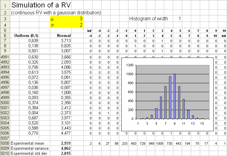
This histogram is interesting because, when properly rescaled, it is an approximation of the density of probability of the random variable X. We know that X has a bell shape frequency distribution - because that's how we produced 20 outcomes of X with the Excel simulation sheet. We can produce very easily 5000 outcomes of X, and plot the histogram directly with Excel. Here is a result :

(Caution : on this picture, the numbers of the horizontal axis of the histogram plotted by Excel are the ranks of the intervals.)

We see now a nice bell shape curve showing up. Its experimental mean is between the 8th and the 9th interval, that is, around 3. Calculation yields : 2,931.

And it has a "width", which correspond to the spread, or the variability, of X around its mean. Now is time to define this concept.

Variance and standard deviation

Some random variable have a large variability around their mean, and some have a small variability around their mean. Some even have no variability around their mean ; in truth they are not random variables, they are fixed numbers.

We are very much concerned with the variability of random variables around their mean, because, in finance, it will make a big difference to us to invest 100 € and expect 120 € with a small possible variability, or expect 120 € with a wide possible variability. The limit case of "small variability" is no variability at all. If we can find an investment where we put up 100 € today, and get for sure 120 € in one year, this is a great investment because the risk free rate offered in the euro zone, at the moment, is only 2% (and not 20% !). In short, it is not a realistic example. But it is a realistic situation to invest 100 € today, and expect 120 € in one year, if this payoff in one year has a significant variability. (The variability we talk about in these lectures, when we talk about securities traded in the stock market, is the so-called "systematic variability linked to the randomness of the economy" ; it is not a "specific variability" similar to that produced by a random generating device. Only the full fledged theory of securities explains this in detail.)

Remember that investors are "risk averse". For two securities S and T, both promising, on average, 120 € in one year, they will pay more for the one that has the least variability. The limit case, once again, is no variability at all, in which case, in October 2005, the market price of such a security today is 117,65 €. But a security promising 120 € in one year with variability around this mean value, may well have a market price of only 100 €, or even less. Only market data in October 2005, for various variabilities, will give us the price for a given security.

To grasp the idea of risk aversion, here is a striking example. Suppose we have the choice between two games :

• game 1 : we receive for sure, in one year, 100 000 €
• game 2 : in one year, we receive either 200 000€ or 0 €, with probabilities 50%-50%.

Both games have the same expected gain. Yet, most of us will prefer game 1. And, if we must pay to play the game, we will pay more for game 1 than for game 2. For game 1, any price below 98 040 € is a good price for us, because there are people who will, then, buy from us, today, the game ticket for 98  040 €. But for game 2, different people will pay different prices, according to their attitude toward money. (Note that only in game 2, you have the possibility to gain 200 000 €...)

The way we shall measure the variability of a random variable X is by looking at the second random variable [X - E(X)]². It is the "squared deviation of X around its mean". If X varies a lot, the outcomes of [X - E(X)]² will often be big. Whereas if X doesn't vary a lot, [X - E(X)]² will stay small.

Definition : we define the variance of X as the expectation of [X - E(X)]². And we denote it Var(X).

The definition of the standard deviation of X (in French, "écart type de la variable aléatoire X") is simply the square root of the variance of X.

Examples :

Let's begin with discrete random variables :

X has the following possible outcomes and probabilities :

Clearly, E(X) = 100. Computation yields Variance of X = 200, and, therefore, std dev (X) = 14,14.

Y has the following possible outcomes and probabilities :

E(Y) = 100. Variance of Y = 120, and std dev (Y) = 10,95.

Z has the following possible outcomes and probabilities (it is like Y shifted by 15) :

E(Z) = 115. Variance of Z = 120, and std dev (Z) = 10,95.

For continuous random variables, the calculation of E(X) and Var(X) requires calculus. But we shall only deal with normal random variables in this course, and we can always do simulations to get a feel for the behavior of the random variables.

We already saw that the mean of a Gaussian random variable with parameters μ and σ, that is, with the density of probability

is E(X) = μ.

It turns out that the variance of X is σ², or, equivalently, the standard deviation of X is σ.

Put another way : a Gaussian distribution is entirely specified by its mean and standard deviation. And the formula for the density of probability can be expressed with these two attributes. That's why, when we talk about a Gaussian random variable, we only specifiy its mean and standard deviation.

Exercise : construct an Excel sheet to simulate a Gaussian random variable (with mean 10 and standard deviation 18) and check that the experimental mean of a large number of trials is not far from 10, and the experimental standard deviation is not far from 18. (Use the tool Simulation_normal.xls constructed in class.)

break time

Go to part 2