Wednesday November 24th 2004
Finance : lesson seven.
Introduction
One security S
Random walks
Google
Security S (cont'd)
Histogram
The spread of X
A representation of S and its variability
Another security T
Is T less or more risky than S ?
Market price for T
Exercise on variability
Why don't we use prices to define risk pattern ?
Use of the concept of risk pattern
A note on mathematical notations
Investments with several future cash flows
The school, at the last minute, decided to cancel today's examination, and to move it next week. In every unfortunate circumstance there is something positive to gain : instead of shooting for 95% of students mastering the topics so far, we will review once more together and shoot for 100%.
Exercise : Let's make up a security S with some price today, an expected value in one year, and a profitability of 20%.
Answer :
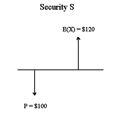
Let's choose, for instance, P today = $100.
Let's call X the random value of S in one year. Then we want E(X) to be such that S yields a profitability 20%, so E(X) must be $120.
We could also have chosen P = $68 and E(X) = $81,6. Any two numbers such that the second one is 1,2 times the first one would have done. But let's stick to simple numbers, with an initial price of $100. It is simpler for the calculations.
The standard graphical representation of S is this

Now, let's make sure we understand very well what we just constructed.
E(X) is the mean of a random variable X. The actual value of S in one year will be an outcome of X. Let's imagine that we can reproduce several times "waiting one year" after having purchased S for a price P. A series of outcomes of X can be
| 134 |
| 152 |
| 94 |
| 120 |
| 120 |
| 152 |
| 159 |
| 97 |
| 118 |
| 71 |
It is fundamental to understand that these are not an example of ten successive values of S over ten years.
Successive values of S year after year, in the standard model in Finance, form a random walk. Each value, although random, depends upon the preceding one. The usual model is
Xn+1 = Xn * (1 + Rn+1)
where the Rn's are independent random profitabilities with the same distribution.
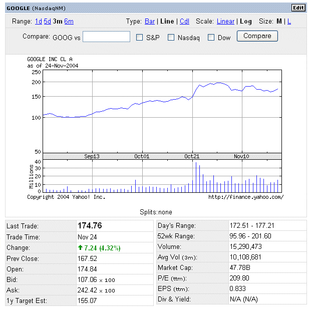
Google stock, like any other stock, is a nice example of random walk. It is a particularly exciting one because it is one of the new stars of the NASDAQ (the US stock market for technology stocks).
Google stock
lost a few percent, to $165, after this press announcement
Google Founders Sell Stock
 According
to
SiliconValley.com, Larry Page and Sergey Brin each plan to sell up to 7.2
million shares of their stock in the online search engine leader during the
next 18 months.
Based on current prices, Page and Brin would each pocket $1.2 billion from
their planned stock sales.
But then it went up again.
Note that this sale of shares by the founders will not bring money into Google's bank account, only into the founders' pockets. It is an example of the secondary function of the stock market : exchange of stocks and money between stock market players. (The first function of the stock market is to bring money into firm's when firms sell new shares.)
Note that at the current share price of $174.76 the total "market value" (also called "market capitalisation") of Google is $47.78 billions. It is the current price of one share multiplied by the number of shares held by stockholders. Most of these shares have not yet been traded in the stock market. They were created at the beginning of Google, 6 years ago.
Do not mix up money and value. The value of Google nowadays can be said to be $47 billions, although it is not very significant until someone pays this sum in money to buy it.
There is one firm that would be interested. And it has almost all the cash necessary. Do you know which one ? To be precise this potential buyer has the value readily transformable into cash. Nobody keeps $47 billions in cash ! One puts it into Treasury bonds and other sure and liquid values.
I repeat : let's not mix up money and value. Money is "the blood" of the economy. There is much less money than the values created and exchanged every year. And in fact if someone kept huge amounts of money idle, it would diminish the "money supply" and create problems in the economy.
The safety of the value of money (that is the purchasing power of money) is also an important question.
It is my forecast that in 20 years, there will be only two important currencies in the World : the Euro and the Yuan. To make a strong currency you need two conditions :
In the meantime we will have lived through much turmoil.
Back to learning the basics.
In the example of this lesson we are thinking only of the outcome next year of X, not a sequence of years. We reproduce "in our head" the act of waiting until next year, and therefore we can think of ten outcomes of X.
The ten numbers we chose are quite interesting.
We could have chosen
| 120 |
| 120 |
| 120 |
| 120 |
| 120 |
| 120 |
| 120 |
| 120 |
| 120 |
| 120 |
This would have been the ten outcomes of a US Treasury bond worth $120 in one year !
Indeed we know that only Treasury bonds have a sure value in one year. And US Treasury bonds as of November 2004 yield 1,75%. (I'm simplifying life a bit. The mentioned rate is for very short lending to the Fed. But the gist is correct.) So the price today ought to be
120/(1+1,75%) = $117,9
So this would not have been an adequate example. And indeed we chose a series of outcomes that show some variability.
First of all let's compute the estimated expectation of X from our ten outcomes :
estimated E(X) = (134 + 152 + 94 + ... + 118 + 71)/10 = $121,7
It's not 120. It does not have to be exactly 120. But it is not far. Fine !
Let us plot the data we produced
| 134 |
| 152 |
| 94 |
| 120 |
| 120 |
| 152 |
| 159 |
| 97 |
| 118 |
| 71 |
As we already saw in lesson 4a, the first graph that comes to mind is this one :
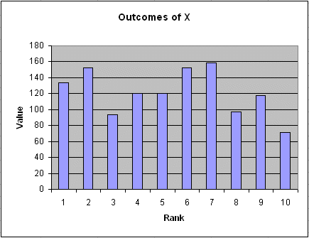
It is just the simple plot of each data : along the abscissa its rank, along the ordinate its value.
But this plot is not very interesting. It carries useless information : the fact that the outcome $152 was the sixth one is irrelevant ; it could have been the fourth, or the ninth, the information for us would be the same.
What is important is "how many outcomes" fell in each horizontal slice along the vertical axis. We have to choose the slices we want to use : let's use slices $20 wide. Then the counts are :
in slice $60 < X
≤ $80 : one outcome
in slice $80 < X ≤ $100 : two
outcomes
in slice $100 < X ≤ $120 : three
outcomes
in slice $120 < X ≤ $140 : one
outcome
in slice $140 < X ≤ $160 : three
outcomes
Then we plot the "histogram" (which is equivalent to a flip around the 45° diagonal of the above graph, followed by a count in each vertical slice)
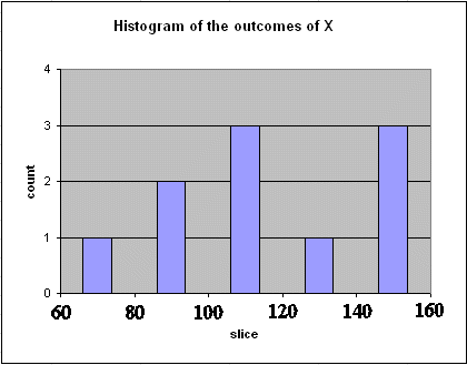
This graph not only suggests that the mean of X is around $120, but also it begins to show the spread of X.
Of course we would have a much better view of the distribution of X among all the slices if we had more data than just ten. If we had, say, a couple hundred data we would begin to see well the actual frequency distribution of X, most usually in Finance it is a bell shape curve.
The spread of a random variable is defined as its standard deviation. The standard deviation is the square root of the variance. And the variance is defined as the mean of the squared deviation of any outcome of X from the mean of X (this is a casual wording).
So the variance of X can be estimated from the ten data we have. Let's compute the ten squared deviations :
(134 -121,7)2 = 151,29
(152 -121,7)2 = 918,09
...
(71 - 121,7)2 = 2570,49
The average of these ten numbers is Estimated Variance of X = 734,61
Then Estimated Standard Deviation of X = $27,1
This figure is a measurement of the spread of the ten numbers we produce for the value in one year of our security S.
A representation of S and its variability :
A first representation of S and its variability that comes to mind is this. But this is a bad representation.
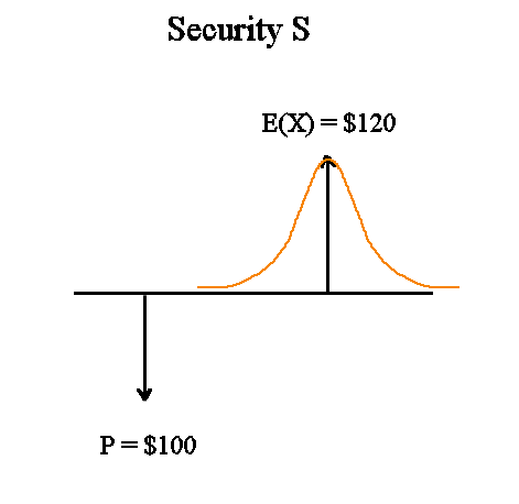
It is a bad representation, because
So we prefer this better representation :
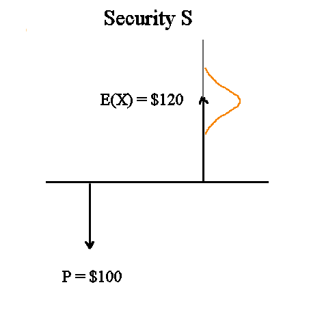
It still mixes up time and density on the horizontal axis but there is less risk of confusion.
Now let's produce another security T with the following conditions :
Let's call Y the random value of T in one year. Since T must have profitability 20%, E(Y) must be $33,333 * 1,2 = $40
Let's produce ten values of Y, and let's try to have a different spread from X. Here are ten values :
| 30 |
| 45 |
| 50 |
| 35 |
| 20 |
| 55 |
| 38 |
| 44 |
| 52 |
| 46 |
Their mean is $41,5. That is the Estimated mean of Y is $41,5. Fine !
What about the spread of Y ?
The ten squared deviations of Y around its estimated mean are :
| 132,25 |
| 12,25 |
| 72,25 |
| 42,25 |
| 462,25 |
| 182,25 |
| 12,25 |
| 6,25 |
| 110,25 |
| 20,25 |
The average of these ten numbers is 105,25. It is the estimated variance of Y.
So the estimated standard deviation of Y is $10,26.
Is T less of more risky than S ?
Y has an estimated std dev of $10,26 compared to X which has an estimated std dev of $27,1.
But let's not be mislead : T (or Y) has more variability than S (or X). The comparison should be made after a rescaling. In absolute T varies less, but T is three times cheaper.
What matters is the variability of $100 invested into S compared to $100 invested into T.
To invest $100 into T means "buying three T's". Then the standard deviation of the value of our investment one year later is 3*$10,26 = $30,78. This is more than the variability of investing into S.
So T is more variable.
Or, said equivalently, the risk pattern of S is narrower than the risk pattern of T.
Remember : the absolute figures (price, future value, standard deviation of future value) of a security matter less than the relative figures. For instance if we are excited by Google, we shall not invest into only one stock, we shall invest say $1000. At a price of $165, this will buy us 6 shares (and leave us an extra $10). All our calculations will be made on $1000, or $990, not on $165.
Secondly, we can talk about the future risk behavior of a security even before there exists a price for it.
The securities with the least risk pattern are the Treasury bonds, the values of which in one year have no variability.
If we represent on the same graph S and 3T's, and their distributions, we get this :
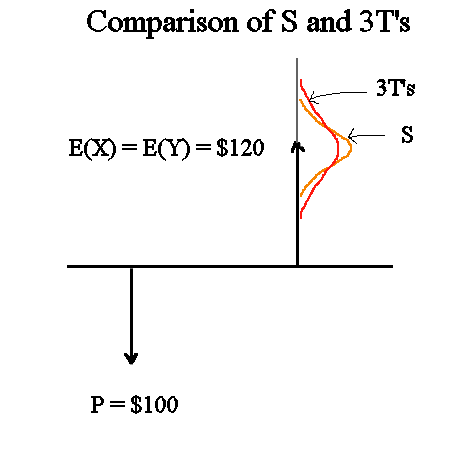
The risk pattern of T is defined as std dev(Y)/E(Y). With the estimations we calculated this gives 24,7%.
The risk pattern of S is estimated to be est sd(X)/est E(X) = 22,3%. It is less than that of T.
In normal market conditions it is not possible to have two "good" securities with the same profitability and different risk patterns.
For the same expected value in one year, investors are willing to pay more for the security with the lesser risk pattern, the limit being Treasury bonds for which investors, in the United States, are willing to pay the future value discounted by only 1,75%.
This is a fundamental rule of Finance : investors demand more profitability from securities with more risk.
For any security for which they are asked to make a bid, they will try to get an estimate of its future expected value and of its variability, and they will make a price offer in accordance with the fundamental rule of Finance.
If our security S (with its price today of $100 and its expected value in one year of $120) is indeed a security traded in the stock market and belongs to the "optimal" ones, then 3T's having the same expected value and a wider risk pattern will have a smaller price than $100.
The CAPM (Capital Asset Pricing Model) theory, the basics of which we will study after the midterm exam, will tell us how to determine the price of T.
Here are five columns of outcomes of five random variables. They all have the same "underlying true mean", but different spread.
Compute the estimated mean and estimated standard deviation of each.
| 129 | 133 | 160 | 72 | 110 | ||||
| 134 | 153 | 114 | 145 | 130 | ||||
| 149 | 131 | 79 | 108 | 123 | ||||
| 112 | 100 | 99 | 136 | 107 | ||||
| 121 | 101 | 87 | 99 | 141 | ||||
| 123 | 136 | 75 | 112 | 115 | ||||
| 141 | 135 | 137 | 110 | 114 | ||||
| 101 | 114 | 144 | 54 | 111 | ||||
| 132 | 106 | 174 | 163 | 109 | ||||
| 78 | 121 | 110 | 129 | 122 |
Answers :
| estimated mean | 122,0 | 123,0 | 117,9 | 112,8 | 118,2 | ||||
| estimated std dev | 19,65 | 16,63 | 32,72 | 31,15 | 10,26 |
Why don't we use prices to define risk pattern ?
It may seem strange that to measure the risk pattern of a security we don't just use for instance sd(X)/P. This would seem to be a natural definition : the future spread divided by the current price.
But one must understand that we want to evaluate the risk behavior of a security before we decide the price we shall offer for it. So we cannot use the measure sd(X)/P. We must use the elements we have about the security, and these are its future expected value, and the spread of this future value.
That is why we define its risk pattern as sd(X)/E(X).
Secondly, the risk of a security is defined as the standard deviation of its random profitability. Its random profitability is (X - P)/P. This profitability, naturally, is defined only after a price P has been introduced. So the risk of a security has a meaning only after its price is known. Whereas its risk pattern is defined prior to any consideration of price.
Use of the concept of risk pattern :
The concept of risk pattern is important. It is what will enable us to calculate the price we should offer for a new security V we are offered.
When we are offered to purchase a security, and asked to make a bid, we don't know its price, since precisely we are asked to propose one.
How to propose a price ? Like for anything : what do we buy ? The only characteristics of the new security V that we can ask for are its expected future value in one year, and the variability of this random future value.
If we don't even have some idea about these characteristics, we are asked to make an offer for something utterly unknown !
How much will you offer for something that you know nothing about :-) ?
OK, we need to know all we can know or estimate in order to make an offer. As far as securities are concerned all we can know or estimate are its expected future value and its spread. The ratio of the two is called the risk pattern. The lower the risk pattern the higher the price we will offer.
We showed in lesson 4b that to compute the price of V we need to know the profitability rU of a security U with the same risk pattern. This profitability is the opportunity cost of capital of V, and the maximum price we should be willing to pay for V is
PV = E(future value of V)/(1 + rU)
We saw that if we pay more for V we violate the fundamental rule of Finance.
A note on mathematical notations :
Be careful not to confuse "Expectation" and "Estimated".
Usually the expectation of X is denoted E(X). Whereas when we want to specify that we are working on an estimated value of something we denote Est(something).
Mathematical notations are introduced only to shorten English, or because they lend themselves to nice algorithms.
But we must always keep in mind the concepts behind the notations. It is when we start to work on the notations without remembering that we are actually working on ideas expressable in plain English that difficulties begin.
For instance : XIII x VII is the same concept as 13 x 7. But in the first case the multiplication is not obvious unless we know the table of XIII, whereas in the second case Indian mathematicians of the early Middle-Ages devised these notations because they lend themselves to a nice algorithm for multiplying : 13 x 7 = 3 x 7 + 10 x 7 : I multiply 3 x 7, I write down a first 1, I make a note of a 2 that will come with the multiples of ten, then I multiply 7 x 1 (in the rank of the tens), I get a 7, I add the 2 that I recall, I get 9, so the answer is 91 (or XCI).
This multiplication technique, which requires that we know "our multiplication tables", and which we learned in primary school, was invented by Indian mathematicians between 300 and 600 AD (check a History book for details). It was necessary to invent the Indian/Arabic numerals as well, and the zero, to make it operational.
Romans did not multiply the way we do.
Calculus is frightening when we forget the ideas behind notations like ∫a to b f(x)dx. In fact, as I already explained, these notations of Leibniz have the drawback that they invite to all sorts of manipulations on the symbols which are erroneous or meaningless in terms of the ideas that they express.
Another example of forgetting the ideas behind the notations is this : suppose we have an object f that is such that
f = limit of fn when n increases
(for example : 2 = limit of 1 + 1/2 + 1/4 + 1/8 + ... + 1/2n , when n increases,
or, the function sin(x) = limit of
x
x-x3/6
x-x3/6+x5/120
x-x3/6+x5/120-etc.
(we take only odd powers, alternate the signs, and the dividing factor of x2n+1 is the product of the integers from 1
to 2n+1) )
then suppose we are interested in applying an operator Φ on f. We want to work with Ξ = Φ { f }. We naturally, and correctly, write Ξ = Φ { limit of fn }. But then we may automatically, and without thinking, write Ξ = limit of Φ { fn }. However, this last equality, if Ξ is already well defined, is definitely not necessarily correct. It is an example of manipulating notations without paying attention to the ideas they express. On the other hand, sometimes, Ξ = Φ { limit of fn } is not a priori defined, in which case we may like to define it as Ξ = limit of Φ { fn }. With a suitable notion of distance, ie a "topology", this is called "continuous extension".
What we see is that one must not stick slavishly to the notations : it makes life difficult ; but one must always keep in mind the ideas behind : very simple.
It is an erroneous variety of "continuous extension" that lead Adam Smith to say wrong things about the convergence of liberal economies toward optimal states (and puzzled economists for two centuries) : most toys we play with when we are kids (fn) are linear and have simple asymptotic behavior (the operator Φ), so Adam Smith thought that bigger systems (like an economy f) have a behavior that is linear and converges to an optimal state, which is not true. And in fact even very simple toys can display "chaotic" behaviors with new types of dynamic stability, but for some reasons most people don't develop an intuition about these systems (they only had ducks in their bathtub :-) ). When we are on the freeway and the traffic is dense, but still flows, we may be cought in a seemingly strange type of traffic tailback with a sinusoidal regime : these stop and go's are not several unrelated jams but only one, and its occurence obeys complex laws.
Overcoming difficulty in mathematics is most of the time only a matter of practice to gain familiarity and experience with the concepts. For those of you who will go farther into sciences (financial or else), you will also have to distinguish between perceptions and ideas. Surprisingly enough, ideas don't always come from perceptions, often it is the other way around. Understanding this gives a great freedom of creativity. For instance representing a complex dynamic system in its phase space becomes as natural as representing it with more usual variables in the space tracking its parts. The study of complex dynamic systems and their convergence toward attractors, that are suboptimal from the viewpoint of classical economics, will resolve questions that have agitated economists for two centuries.
Investments with several future cash flows :
In this second review session before the midterm examination, it is now time to do some exercises concerning investments that will produce cash flows over several years.
Here is such an investment I :
Initial money to be spent C0 = 1000€. Then 4 cash flows produced, with the
following expected values :
C1 = 300€
C2 = 400€
C3 = 200€
C4 = 200€
Is I a good investment ?
The first thing we can say is that it does not look very good : over 4 years, we barely get our money back.
But let's compute the NPV(I ; r) for various values of r.
For r = 5%, we get NPV(I ; 5%) = -14,17€
So, as we learned in lesson 5a, investment I must have a risk behavior lesser than that of securities yielding 5%. And we know that such securities are already not very risky, because their yield is not very far from that of Euro Treasury bonds.
In order to figure out whether I is an acceptable investment, we need to know the risk pattern of I and find the profitability of securities with similar risk pattern. As we explained in lesson 5a, to evaluate the risk pattern of a series of random cash flows is not as easy as for one-cash-flow securities, but we assume that the intuitive idea is clear and sufficient : it is the risk pattern of "similar securities in term of risk". (To avoid this somewhat circular definition requires either to go into intricate financial considerations that are outside the scope of this course, or to make abusively simplistic assumptions about the random behavior of the future cash flows.)
Suppose that the random behavior of the four future CF's of I gives it a risk pattern equivalent to that of securities yielding 4% in the stock market. Then 4% is the opportunity cost of capital of I.
NPV(I) = NPV(I ; 4%) = + 7,04€
So I is an acceptable investment.
Equivalently, let's compute the value r for which NPV(I ; r) = 0. It is by definition its IRR. Remember to note that the IRR is an internal figure of I, it does not refer to any outside security or anything. Trial and error, or geometric interpolation between 4% and 5%, yields
IRR(I) = 4,33%
Two equivalent ways to evaluate an investment I :